A Real-time Retrieval System for RAG on Social Media Data

Use a streaming engine to populate a vector DB in real time. Use rerank & UMAP to improve the accuracy of your retrieved documents.

Mar 07, 2024

We are putting in a lot of time to create high-quality content. Thus, we want to make it as convenient as possible for you to read our content.
That is why we will experiment with the posting time and move it to Thursday at 3:00 PM CET.

In this article, you will learn how to build a real-time retrieval system for social media data. In our example, we will use only my LinkedIn posts, but our implementation can easily be extended to other platforms supporting written content, such as X, Instagram, or Medium.

In this article, you will learn how to:

build a streaming pipeline that ingests LinkedIn posts into a vector DB in real-time
clean, chunk, and embed LinkedIn posts
build a retrieval client to query LinkedIn posts
use a rerank pattern to improve retrieval accuracy
visualize content retrieved for a given query in a 2D plot using UMAP

Our implementation focuses on just the retrieval part of an RAG system. But you can quickly hook the retrieved LinkedIn posts to an LLM for post analysis or personalized content generation.

Because LinkedIn posts (or any other social media data) evolve frequently, your vector DB can quickly get out of sync. To handle this, you can build a batch pipeline that runs every minute. But to really minimize data lag, to make sure your vector DB stays current with new social media posts, you need to use a streaming pipeline that immediately takes every new item the moment it's posted, preprocesses it, and loads it into the vector DB.

Why Bytewax?

Bytewax is a streaming engine built in Rust that exposes a Python interface. We use Bytewax because it combines the impressive speed and reliability of Rust with the ease of use and ecosystem of Python.

1.2. The retrieval client

Our retrieval client is a standard Python module that preprocesses user queries and searches the vector DB for most similar results. Qdrant vector DB lets us decouple the retrieval client from the streaming ingestion pipeline.

Using a semantic-based retrieval system lets us query our LinkedIn post collection very flexibly. For example, we can retrieve similar posts using a variety of query types - e.g., posts, questions, sentences.

Also, to improve the retrieval system's accuracy, we use a rerank pattern.

Lastly, to better understand and explain the retrieval process for particular queries, we visualize our results on a 2D plot using UMAP.

2. Data

We will ingest 215 LinkedIn posts from my Linked profile - Paul Iusztin. Though we simulate the post ingestion step using JSON files, the posts themselves are authentic.

Before diving into the code, let's take a look at an example LinkedIn post to familiarize ourselves with the challenges it will introduce ↓

[
    {
        "text": "𝗪𝗵𝗮𝘁 do you need to 𝗳𝗶𝗻𝗲-𝘁𝘂𝗻𝗲 an open-source 𝗟𝗟𝗠 to create your own 𝗳𝗶𝗻𝗮𝗻𝗰𝗶𝗮𝗹 𝗮𝗱𝘃𝗶𝘀𝗼𝗿?\nThis is the 𝗟𝗟𝗠 𝗳𝗶𝗻𝗲-𝘁𝘂𝗻𝗶𝗻𝗴 𝗸𝗶𝘁 you must know ↓\n𝗗𝗮𝘁𝗮𝘀𝗲𝘁\nThe key component of any successful ML project is the data.\nYou need a 100 - 1000 sample Q&A (questions & answers) dataset with financial scenarios.\nThe best approach is to hire a bunch of experts to create it manually.\nBut, for a PoC, that might get expensive & slow.\nThe good news is that a method called \"𝘍𝘪𝘯𝘦𝘵𝘶𝘯𝘪𝘯𝘨 𝘸𝘪𝘵𝘩 𝘥𝘪𝘴𝘵𝘪𝘭𝘭𝘢𝘵𝘪𝘰𝘯\" exists.\n 
...
Along with ease of deployment, you can easily add your training code to your CI/CD to add the final piece of the MLOps puzzle, called CT (continuous training).\n↳ Beam: 🔗\nhttps://lnkd.in/dedCaMDh\n.\n↳ To see all these components in action, check out my FREE 𝗛𝗮𝗻𝗱𝘀-𝗼𝗻 𝗟𝗟𝗠𝘀 𝗰𝗼𝘂𝗿𝘀𝗲 & give it a ⭐:  🔗\nhttps://lnkd.in/dZgqtf8f\nhashtag\n#\nmachinelearning\nhashtag\n#\nmlops\nhashtag\n#\ndatascience",
        "image": "https://media.licdn.com/dms/image/D4D10AQHWQzZcToQQ1Q/image-shrink_800/0/1698388219549?e=1705082400&v=beta&t=9mrDC_NooJgD7u7Qk0PmrTGGaZtuwDIFKh3bEqeBsm0"
    }
]

The following features of the above post are not compatible with embedding models. We'll need to find some way of handling them in our preprocessing step:

emojis
bold, italic text
other non-ASCII characters
URLs
content that exceeds the context window limit of the embedding model

Emojis and bolded and italic text are represented by Unicode characters that are not available in the vocabulary of the embedding model. Thus, these items cannot be tokenized and passed to the model; we have to remove them or normalize them to something that can be parsed by the tokenizer. The same holds true for all other non-ASCII characters.

URLs take up space in the context window without providing much semantic value. Still, knowing that there's a URL in the sentence may add context. For this reason, we replace all URLs with a [URL] token. This lets us ingest whatever value the URL's presence conveys without it taking up valuable space.

3. Streaming ingestion pipeline

Let's dive into the streaming pipeline, starting from the top and working our way to the bottom ↓

3.1. The Bytewax flow

The Bytewax flow transparently conveys all the steps of the streaming pipeline.

The first step is ingesting every LinkedIn post from our JSON files. In the next steps, every map operation has a single responsibility:

validate the ingested data using a RawPost pydantic model
clean the posts
chunk the posts; because chunking will output a list of ChunkedPost objects, we use a flat_map operation to flatten them out
embed the posts
load the posts to a Qdrant vector DB

def build_flow():
    embedding_model = EmbeddingModelSingleton()

    flow = Dataflow("flow")

    stream = op.input("input", flow, JSONSource(["data/paul.json"]))
    stream = op.map("raw_post", stream, RawPost.from_source)
    stream = op.map("cleaned_post", stream, CleanedPost.from_raw_post)
    stream = op.flat_map(
        "chunked_post",
        stream,
        lambda cleaned_post: ChunkedPost.from_cleaned_post(
            cleaned_post, embedding_model=embedding_model
        ),
    )
    stream = op.map(
        "embedded_chunked_post",
        stream,
        lambda chunked_post: EmbeddedChunkedPost.from_chunked_post(
            chunked_post, embedding_model=embedding_model
        ),
    )
    op.inspect("inspect", stream, print)
    op.output(
        "output", stream, QdrantVectorOutput(vector_size=model.embedding_size)
    )
    
    return flow

3.2. The processing steps

Every processing step is incorporated into a pydantic model. This way, we can easily validate the data at each step and reuse the code in the retrieval module.

We isolate every step of an ingestion pipeline into its own class:

cleaning
chunking
embedding

Doing so, we follow the separation of concerns good SWE practice. Thus, every class has its own responsibility.

Now the code is easy to read and understand. Also, it’s future-proof, as it’s extremely easy to change or extend either of the 3 steps: cleaning, chunking and embedding.

Here is the interface of the pydantic models:

class RawPost(BaseModel):
    post_id: str
    text: str
    image: Optional[str]

    @classmethod
    def from_source(cls, k_v: Tuple[str, dict]) -> "RawPost":
        ... # Mapping a dictionary to a RawPost validated pydantic model.

        return cls(...)

class CleanedPost(BaseModel):
    post_id: str
    raw_text: str
    text: str
    image: Optional[str]

    @classmethod
    def from_raw_post(cls, raw_post: RawPost) -> "CleanedPost":
        ... # Cleaning the raw post

        return cls(...)


class ChunkedPost(BaseModel):
    post_id: str
    chunk_id: str
    full_raw_text: str
    text: str
    image: Optional[str]

    @classmethod
    def from_cleaned_post(
        cls, cleaned_post: CleanedPost, embedding_model: EmbeddingModelSingleton
    ) -> list["ChunkedPost"]:
        chunks = ... # Compute chunks

        return [cls(...) for chunk in chunks]


class EmbeddedChunkedPost(BaseModel):
    post_id: str
    chunk_id: str
    full_raw_text: str
    text: str
    text_embedding: list
    image: Optional[str] = None
    score: Optional[float] = None
    rerank_score: Optional[float] = None

    @classmethod
    def from_chunked_post(
        cls, chunked_post: ChunkedPost, embedding_model: EmbeddingModelSingleton
    ) -> "EmbeddedChunkedPost":
        ... # Compute embedding.

        return cls(...)

Now, the data at each step is validated and has a clear structure.

Note: Providing different types when instantiating a pydantic model will throw a validation error. For example, if the post_id is defined as a string, and we try to instantiate an EmbeddedChunkedPost with a None or int post_id, it will throw an error.

Check out the full implementation on our 🔗 GitHub Articles Hub repository.

3.3. Load to Qdrant

To load the LinkedIn posts to Qdrant, you have to override Bytewax's StatelessSinkPartition class (which acts as an output in a Bytewax flow):

class QdrantVectorSink(StatelessSinkPartition):
    def __init__(
        self,
        client: QdrantClient,
        collection_name: str
    ):
        self._client = client
        self._collection_name = collection_name

    def write_batch(self, chunks: list[EmbeddedChunkedPost]):
        ... # Map chunks to ids, embeddings, and metadata.

        self._client.upsert(
            collection_name=self._collection_name,
            points=Batch(
                ids=ids,
                vectors=embeddings,
                payloads=metadata,
            ),
        )

Within this class, you must overwrite the write_batch() method, where we will serialize every EmbeddedChunkedPost to a format expected by Qdrant and load it to the vector DB.

4. Retrieval client

Here, we focus on preprocessing a user's query, searching the vector DB, and postprocessing the retrieved posts for maximum results.

To design the retrieval step, we implement a QdrantVectorDBRetriever class to expose all the necessary features for our retrieval client.

class QdrantVectorDBRetriever:
    def __init__(
        self,
        embedding_model: EmbeddingModelSingleton,
        vector_db_client: QdrantClient,
        cross_encoder_model: CrossEncoderModelSingleton
        vector_db_collection: str
    ):
        self._embedding_model = embedding_model
        self._vector_db_client = vector_db_client
        self._cross_encoder_model = cross_encoder_model
        self._vector_db_collection = vector_db_collection

    def search(
        self, query: str, limit: int = 3, return_all: bool = False
    ) -> Union[list[EmbeddedChunkedPost], dict[str, list]]:
        ... # Search the Qdrant vector DB based on the given query.

    def embed_query(self, query: str) -> list[list[float]]:
        ... # Embed the given query.

    def rerank(self, query: str, posts: list[EmbeddedChunkedPost]) -> list[EmbeddedChunkedPost]:
        ... # Rerank the posts relative to the given query.

    def render_as_html(self, post: EmbeddedChunkedPost) -> None:
        ... # Map the embedded post to HTML to display it.

4.1. Embed query

We must embed the query in precisely the same way we ingested our posts into the vector DB. Because the streaming pipeline is written in Python (thanks to Bytewax), and every preprocessing operation is modular, we can quickly replicate all the steps necessary to embed the query.

class QdrantVectorDBRetriever:

    ...

    def embed_query(self, query: str) -> list[list[float]]:
        cleaned_query = CleanedPost.clean(query)
        chunks = ChunkedPost.chunk(cleaned_query, self._embedding_model)
        embdedded_queries = [
            self._embedding_model(chunk, to_list=True) for chunk in chunks
        ]

        return embdedded_queries

Check out the full implementation on our 🔗 GitHub repository.

4.2. Plain retrieval

Let’s try to retrieve a set of posts without using the rerank algorithm.

vector_db_retriever = QdrantVectorDBRetriever(
    embedding_model=EmbeddingModelSingleton(),
    vector_db_client=build_qdrant_client()
)

query = "Posts about Qdrant"
retrieved_results = vector_db_retriever.search(query=query)
for post in retrieved_results["posts"]:
    vector_db_retriever.render_as_html(post)

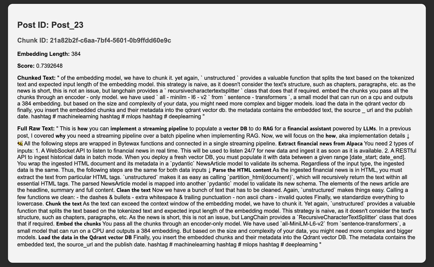
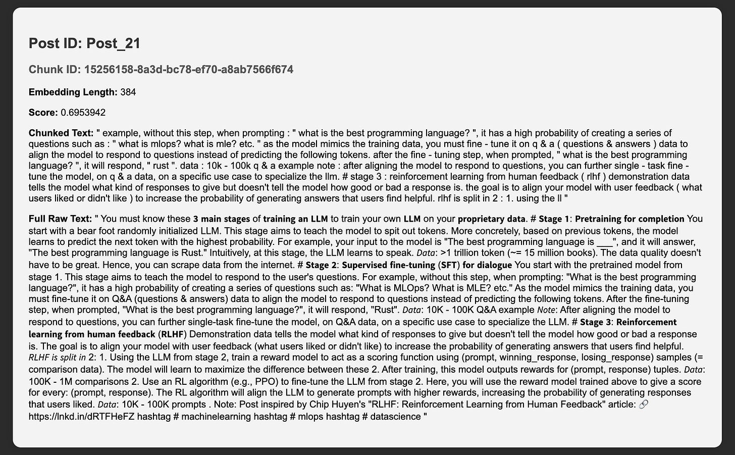
Here are the top 2 retrieved results sorted using the cosine similarity score ↓

Result 1:

Result 2:

You can see from the results above, that starting from the second post the results are irrelevant. Even though it has a cosine similarly score of ~0.69 the posts doesn’t contain any information about Qdrant or vector DBs.

Note: We looked over the top 5 retrieved results. Nothing after the first post was relevant. We haven’t added them here as the article is already too long.

4.3. Visualize retrieval

To visualize our retrieval, we implement a dedicated class that uses the UMAP dimensionality reduction algorithm. We have picked UMAP as it preserves the geometric properties between points (e.g., the distance) in higher dimensions when they are projected onto lower dimensions better than its peers (e.g., PCA, t-SNE).

The RetrievalVisualizer computes the projected embeddings for the entire vector space once. Afterwards, it uses the render() method to project only the given query and retrieved posts, and plot them to a 2D graph.

class RetrievalVisualizer:
    def __init__(self, posts: list[EmbeddedChunkedPost]):
        self._posts = posts

        self._umap_transform = self._fit_model(self._posts)
        self._projected_post_embeddings = self.project_posts(self._posts)

    def _fit_model(self, posts: list[EmbeddedChunkedPost]) -> umap.UMAP:
        umap_transform = ... # Fit a UMAP model on the given posts.

        return umap_transform

    def project_posts(self, posts: list[EmbeddedChunkedPost]) -> np.ndarray:
        embeddings = np.array([post.text_embedding for post in posts])

        return self._project(embeddings=embeddings)

    def _project(self, embeddings: np.ndarray) -> np.ndarray:
        ... # Project the embeddings to 2D using UMAP.

        return umap_embeddings

    def render(
        self,
        embedded_queries: list[list[float]],
        retrieved_posts: list[EmbeddedChunkedPost],
    ) -> None:
      ... # Render the given queries & retrieved posts using matplotlib.

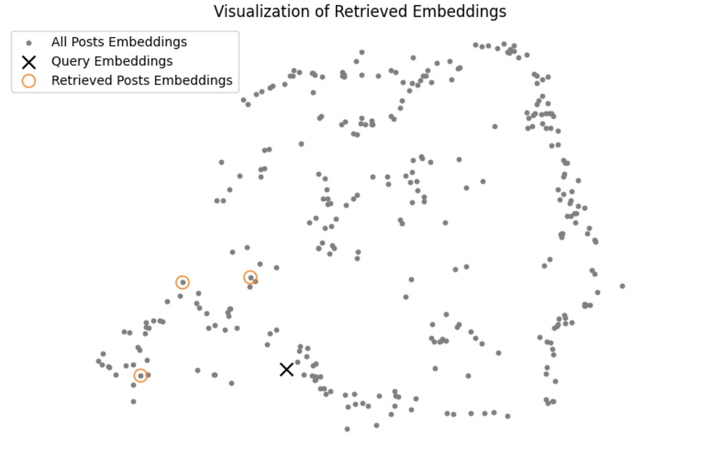
Let's take a look at the result to see how the "Posts about Qdrant" query looks ↓

Visualization of the “Posts about Qdrant” query using UMAP (without reranking) [Image by the Author - in collaboration with VectorHub].

Our results are not great. You can see how far the retrieved posts are from our query in the vector space.

Can we improve the quality of our retrieval system using the rerank algorithm?

4.4. Rerank

We use the reranking algorithm to refine our retrieval for the initial query. Our initial retrieval step - because it used cosine similarity (or similar distance metrics) to compute the distance between a query and post embeddings - may have missed more complex (but essential) relationships between the query and the documents in the vector space. Reranking leverages the power of transformer models that are capable of understanding more nuanced semantic relationships.

We use a cross-encoder model to implement the reranking step, so we can score the query relative to all retrieved posts individually. These scores take into consideration more complex relationships than cosine similarity can. Under the hood is a BERT classifier that outputs a number between 0 and 1 according to how similar the 2 given sentences are. The BERT classifier outputs 0 if they are entirely different and 1 if they are a perfect match.

Bi-Encoder vs. Cross-Encoder [Image by the Author - in collaboration with VectorHub]

But, you might ask, "Why not use the cross-encoder model from the start if it is that much better?"

The answer, in a word, is speed. Using a cross-encoder model to search your whole collection is much slower than using cosine similarity. To optimize your retrieval, therefore, your reranking process should involve 2 steps:

an initial rough retrieval step using cosine similarity, which retrieves the top N items as potential candidates
filtering the rough search using the rerank strategy, which retrieves the top K items as your final results

The implementation is relatively straightforward. For each retrieved post, we create a pair consisting of the (cleaned) query and the text of the post. We do this for all retrieved posts, resulting in a list of pairs.

Next, we call a cross-encoder/ms-marco-MiniLM-L-6-v2 model (from sentence-transformers) to give the retrieved posts their rerank score. We then sort the posts in descending order based on their rerank score.

Check out the rerank algorithm implementation on our 🔗 GitHub repository.

4.5. Visualize retrieval with rerank

Now that we've added the rerank pattern to our retrieval system, let's see if it improves the results of our "Posts about Qdrant" query ↓

Result 1

Result 2:

The improvement is remarkable! All our results are about Qdrant and vector DBs.

Note: We looked over the top 5 retrieved results. The top 4 out of 5 posts are relevant to our query, which is incredible.

Now, let's look at the UMAP visualization:

Visualization of the “Posts about Qdrant” query using UMAP (with reranking) [Image by the Author - in collaboration with VectorHub].

While the returned posts aren't very close to the query, they are a lot closer to the query compared to when we weren't reranking the retrieved posts.

5. Conclusion

In this article, we learned how to adapt a RAG retrieval pattern to improve LinkedIn post retrieval. To keep our database up to date with rapidly changing social media data, we implemented a real-time streaming pipeline that uses CDC to sync the raw LinkedIn posts data source with a vector DB. You also saw how to use Bytewax to write - using only Python - a streaming pipeline that cleans, chunks, and embeds LinkedIn posts.

Finally, you learned how to implement a standard retrieval client for RAG and saw how to improve it using the rerank pattern. As retrieval is complex to evaluate, you saw how to visualize the retrieval for a given query by rendering all the posts, the query, and the retrieved posts in a 2D space using UMAP.

This article is a summary of my contribution from VectorHub. Check out the full article here to dig into the details, the code and more experiments.