Embeddings: the cornerstone of AI & ML
Fundamentals of embeddings: what they are, how they work, why they are so powerful and how they are created.
Embeddings are the cornerstone of many AI and ML applications, such as GenAI, RAG, recommender systems, encoding high-dimensional categorical variables (such as input tokens for LLMs) and more.
For example, in an RAG application, they play a pivotal role in indexing and retrieving data from the vector DB, directly impacting the retrieval step.
They are present in almost every ML field in one form or another.
Thus, having a strong intuition of how embeddings work is a powerful skill.
In this article, you will learn about the fundamentals of embeddings, such as:
what they are
how they work
why they are so powerful
how they are created
What are embeddings
Imagine you're trying to teach a computer to understand the world. Embeddings are like a particular translator that turns these things into a numerical code. This code isn't random, though, because similar words or items end up with codes that are close to each other. It's like a map where words with similar meanings are clustered together.
With that in mind, a more theoretical definition is that embeddings are dense numerical representations of objects encoded as vectors in a continuous vector space, such as words, images, or items in a recommendation system. This transformation helps capture the semantic meaning and relationships between the objects. For instance, in natural language processing (NLP), embeddings translate words into vectors where semantically similar words are positioned closely together in the vector space.
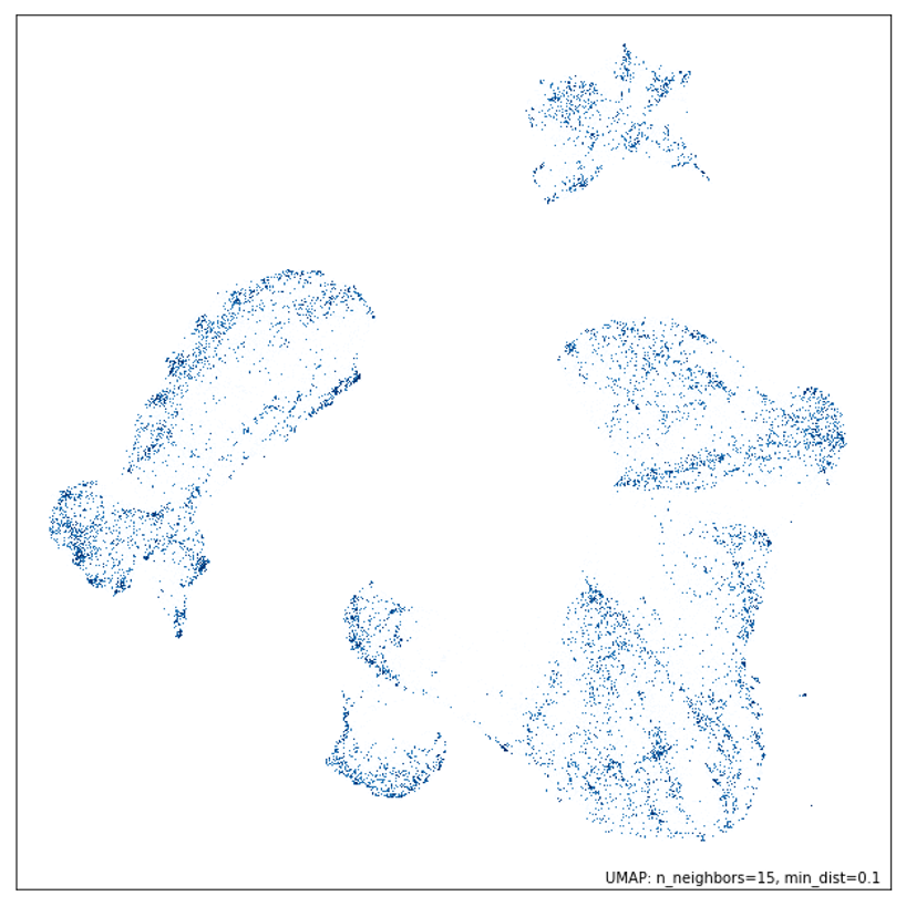
A popular method is visualizing the embeddings to understand and evaluate their geometrical relationship. As the embeddings often have more than 2 or 3 dimensions, usually between 64 and 2048, you must project them again to 2D or 3D.
For example, you can use UMAP, a dimensionality reduction method well known for keeping the geometrical properties between the points when projecting the embeddings to 2D or 3D. Another popular algorithm for dimensionality reduction when visualizing vectors is t-SNE. However, compared to UMAP, it is more stochastic and doesn’t preserve the topological relationships between the points.

Why embeddings are so powerful
First, machine learning models work only with numerical values. This is not a problem when working with tabular data, as the data is often in numerical form or can easily be processed into numbers. Embeddings come in handy when we want to feed words, images or audio data into models.
For instance, when working with transformer models, you tokenize all your text input, where each token has an embedding associated with it. The beauty of this process lies in its simplicity-the input to the transformer is a sequence of embeddings, which can be easily and confidently interpreted by the dense layers of the neural network.
Based on this example, you can use embeddings to encode any categorical variable and feed it to an ML model. But why not use other simple methods, such as one hot encoding? When working with categorical variables with high cardinality, such as language vocabularies, you will suffer from the curse of dimensionality when using other classical methods. For example, if your vocabulary has 10000 tokens, then only one token will have a length of 10000 after applying one hot encoding. If the input sequence has N tokens, that will become in N * 10000 input parameters. If N >= 100, often when inputting text, the input is too large to be usable. Another issue with other classical methods that don’t suffer from the curse of dimensionality, such as hashing, is that you lose the semantic relationships between the vectors.
Secondly, embedding your input reduces the size of its dimension and condenses all of its semantic meaning into a dense vector. This is an extremely popular technique when working with images, where a CNN encoder module maps the high-dimensional meaning into an embedding, which is later processed by a CNN decoder that performs the classification or regression steps.
The image below shows a typical CNN layout. Imagine tiny squares within each layer. Those are the "receptive fields." Each square feeds information to a single neuron in the previous layer. As you move through the network, two key things are happening:
Shrinking the Picture: Special "subsampling" operations make the layers smaller, focusing on essential details.
Learning Features: "Convolution" operations, on the other hand, actually increase the layer size as the network learns more complex features from the image.
Finally, a fully connected layer at the end takes all this processed information and transforms it into the final vector embedding, a numerical image representation.

How are embeddings created?
Embeddings are created by deep learning models that understand the context and semantics of your input and project it into a continuous vector space.
Various deep learning models can be used to create embeddings, varying by the data input type. Thus, it is fundamental to understand your data and what you need from it before picking an embedding model.
For example, when working with text data, one of the early methods used to create embeddings for your vocabulary is Word2Vec and GloVe. These are still popular methods used today for simpler applications.
Another popular method is to use encoder-only transformers, such as BERT, or other methods from its family, such as RoBERTa. These models leverage the encoder of the transformer architecture to smartly project your input into a dense vector space that can later be used as embeddings.
To quickly compute the embeddings in Python, you can conveniently leverage the Sentence Transformers Python package (also available in HuggingFace's transformer package). This tool provides a user-friendly interface, making the embedding process straightforward and efficient.
from sentence_transformers import SentenceTransformer

# 1. Load a pretrained Sentence Transformer model.
model = SentenceTransformer("all-MiniLM-L6-v2")

sentences = ["The dog sits outside waiting for a treat.", "I am going swimming.", "The dog is swimming."]

# 2. Calculate embeddings.
embeddings = model.encode(sentences)
print(embeddings.shape)

# Output: [3, 384]

# 3. Calculate the embedding similarities using cosine similarity.
similarities = model.similarity(embeddings, embeddings)
print(similarities)

# Output:

# tensor([[ 1.0000, -0.0389,  0.2692],
#     [-0.0389,  1.0000,  0.3837],
#     [ 0.2692,  0.3837,  1.0000]])


# similarities[0, 0] = The similarity between the first sentence and itself.
# similarities[0, 1] = The similarity between the first and second sentence.
# similarities[2, 1] = The similarity between the third and second sentence.
The best-performing embedding model can change with time and your specific use case. You can find particular models on the Massive Text Embedding Benchmark (MTEB) on HuggingFace. Depending on your needs, you can consider the best-performing model, the one with the best accuracy or the one with the smallest memory footprint. This decision is solely based on your requirements (e.g., accuracy, hardware, and so on). However, HuggingFace and SentenceTransformer make switching between different models straightforward. Thus, you can always experiment with various options.
When working with images, you can embed them using convolutional neural networks (CNN). Popular CNN networks are based on the ResNet architecture. However, we can't directly use image embedding techniques for audio recordings. Instead, we can create a visual representation of the audio, such as a spectrogram, and then apply image embedding models to those visuals. This allows us to capture the essence of images and sounds in a way computers can understand.
By leveraging models like CLIP, you can practically embed a piece of text and an image in the same vector space. This allows you to find similar images using a sentence as input, or the other way around, demonstrating the practicality of CLIP.
from io import BytesIO

import requests
from PIL import Image
from sentence_transformers import SentenceTransformer

# Load an image with a crazy cat.
response = requests.get(
        "https://github.com/PacktPublishing/LLM-Engineering/blob/main/images/crazy_cat.jpg?raw=true"
    )
image = Image.open(BytesIO(response.content))

# Load CLIP model.
model = SentenceTransformer("clip-ViT-B-32")

# Encode the loaded image.
img_emb = model.encode(image)

# Encode text descriptions.
text_emb = model.encode(
        [
            "A crazy cat smiling.",
            "A white and brown cat with a yellow bandana.",
            "A man eating in the garden.",
        ]
    )
print(text_emb.shape)

# Output: (3, 512)

# Compute similarities.
similarity_scores = model.similarity(img_emb, text_emb)
print(similarity_scores)

# Output: tensor([[0.3068, 0.3300, 0.1719]])
Here, we provided a small introduction to how embeddings can be computed. The realm of specific implementations is vast, but what is important to know is that embeddings can be computed for most digital data categories, such as words, sentences, documents, images, videos, graphs, etc.
It's crucial to grasp that you must use specialized models when you need to compute the distance between two different data categories, such as the distance between the vector of a sentence and of an image. These models are designed to project both data types into the same vector space, such as CLIP, ensuring accurate distance computation.
Applications of embeddings
Due to the generative AI revolution, which uses RAG, embeddings become extremely popular in information retrieval tasks, such as semantic search for text, code, images, and audio and long-term memory of agents.
But before Gen AI, embeddings were already heavily used in:
Representing categorical variables (e.g., vocabulary tokens) that are fed to an ML model.
Recommender system by encoding the users and items and finding their relationship.
Clustering and outlier detection.
Data visualization by using algorithms such as UMAP.
Classification by using the embeddings as features.
Zero-shot classification by comparing the embedding of each class and picking the most similar one.
Conclusion
In this article, we explored the fundamentals of embeddings.
By grasping an intuition about embeddings, we understood why they are a fundamental skill for any ML engineer. They are the cornerstone of almost any ML application, such as GenAI, RAG and recommender systems projects.
This article was inspired by my latest book, “LLM Engineer’s Handbook.”
If you liked this article, consider supporting my work by buying my book and getting access to an end-to-end framework on how to engineer LLM & RAG applications, from data collection to fine-tuning, serving and LLMOps:

Images
If not otherwise stated, all images are created by the author.


