


The second lesson of the open-source course Building Your Second Brain AI Assistant Using Agents, LLMs and RAG — a free course that will teach you how to architect and build a personal AI research assistant that talks to your digital resources.
A journey where you will have the chance to learn to implement an LLM application using agents, advanced Retrieval-augmented generation (RAG), fine-tuning, LLMOps, and AI systems techniques.
Lessons:
Lesson 1: Build your Second Brain AI assistant
Lesson 2: Data pipelines for AI assistants
Lesson 3: From noisy docs to fine-tuning datasets
Lesson 4: Playbook to fine-tune and deploy LLMs
Lesson 5: Build RAG pipelines that actually work
Lesson 6: LLMOps for production agentic RAG
🔗 Learn more about the course and its outline.
Data pipelines for AI assistants
Welcome to Lesson 2 of Decoding ML’s Building Your Second Brain AI Assistant Using Agents, LLMs and RAG open-source course, where you will learn to architect and build a production-ready Notion-like AI research assistant.
Every data and AI system starts with data. If you don’t have data, you don’t have the raw material to work with. You can have the most fancy algorithms, but without data, they are still like a car without fuel.
Hence, this lesson will teach us to architect and build the data pipelines that fuel our Second Brain AI assistant, such as the Notion data collection and ETL data pipelines.
While implementing the data pipelines, we will learn the following:
Use an MLOps framework such as ZenML to manage the ML pipelines.
Read documents from Notion.
Structure and validate our documents using Pydantic.
Crawl ~400 links found in the Notion documents using Crawl4AI.
Compute quality scores for each document using a two-stage design based on heuristics and LLMs.
Normalize all the documents to Markdown.
Store all the standardized documents in MongoDB.

Let’s get started. Enjoy!
Podcast version of the lesson
Table of contents:
Architecting data pipelines for AI systems
Understanding MLOps frameworks for managing ML pipelines
Exploring the collected Notion data
Looking into requirements for crawling
Implementing crawling
Computing the quality score
Loading the standardized data to a document database
Running the code
1. Architecting data pipelines for AI systems
In most use cases, a data pipeline starts with raw data collection, undergoes some transformation steps, and ultimately loads the transformed data into storage.
To build our Second Brain AI assistant, we must collect data from Notion, crawl all the links found in the Notion documents, and standardize everything in Markdown so downstream processes can easily process the documents.
To implement that, we split the data pipelines into two main components, making the architecture flexible and scalable.
The data collection pipeline
Which uses Notion’s API to access our personal data programmatically. Then, it extracts all the links from the crawled documents and adds them to their metadata. Ultimately, it standardizes the document into Markdown, saves it as JSON, and loads the results in S3.
Forcing people to use their Notion collections wasn’t a scalable solution or a good user experience, and neither was making our Notion collection public.
Thus, we decided to save our processed Notion collection into a public S3 bucket, which everyone can access effortlessly.
To draw a parallel to the industry, the S3 bucket could be seen as a data lake, where multiple teams from the organization push raw data that can be used within the company.
The course will start with reading our custom Notion collection from S3 and the next steps in processing. However, if you want a personalized experience, we provide the code and instructions for collecting your Notion collections.
Thus, let’s dig into the ETL data pipeline, where most of our focus will be.
The ETL data pipeline
ETL stands for “Extract, Transform, Load,” a popular data engineering pattern applied to most data pipelines.
The pattern is simple. You have to extract data from a source, apply some transformations, and ultimately load it into storage that makes the processed data accessible.
Here is how it looks to us:
Extract storage: S3
Transformations: crawling, standardization to Markdown, computing a quality score
Load storage: MongoDB
Now, let’s dig into the details of each step.
Once the data has been downloaded from S3, we want to enrich it by crawling all the links within the Notion documents. This makes sense for two core reasons:
When you chat with your AI assistant, you are primarily curious about what’s inside the link, not the link itself.
We have more data for fine-tuning our summarization LLM.
After the documents are crawled, they are standardized to Markdown format (as well) and added to our existing collection.
We track the source of each document within the metadata, and because the documents are in Markdown format regardless of their source, we can treat the Notion and crawled documents equally and store them in the same collection. This will make our lives 100 times easier during future processing steps.
Formatting everything in Markdown is critical because it ensures the data is standardized and more straightforward to process downstream in the pipeline. This standardization is very important because the data will later be used for RAG (Retrieval Augmented Generation) and to fine-tune a summarization large language model (LLM).

Now that the data has been augmented, ensuring its quality is essential. We compute a quality score for each document. This quality score is a number between 0 and 1, which you can use to filter the documents based on the target quality you are looking for.
You know the famous saying regarding AI systems: “Trash in, trash out.”
Hence, this is a critical step for fine-tuning high-quality LLMs and doing RAG correctly.
We want to filter the data differently depending on whether we use it for RAG or fine-tuning. Thus, we store all documents with the quality score in the metadata. This allows downstream pipelines to decide what to filter.
Ultimately, the standardized data is loaded into a document database and ready for consumption by the feature pipelines, which will further process it for RAG and fine-tuning.
It is a good practice to create a snapshot of the data between the data and AI layers. This decouples the two, allowing you to run the data pipeline once and experiment further with your AI architecture. You can extend this by versioning your data sources and making the data available across your company (instead of just your project).
As before, to draw a parallel to the industry, this is similar to how a data warehouse, such as Big Query, connects the dots between the data and AI systems.
The last piece of the puzzle is our MLOps framework. For our use case, we picked ZenML. Through ZenML, we will manage all our offline pipelines, such as the data collection, ETL pipeline and feature engineering pipelines.
But why do we need an MLOps framework in the first place? Let’s dig into this in the next section.
2. Understanding MLOps frameworks for managing ML pipelines
MLOps frameworks are powerful tools that allow you to easily manage, schedule, track, and deploy your ML pipelines.
Metaflow and ZenML are popular MLOps frameworks. They are optimized for long-running ML jobs, tracking metadata and output artifacts for reproducibility and setting up complex environments required for training and inference.
One core component of these MLOps frameworks is orchestrating offline ML pipelines. There is a fine line between data and ML orchestrators. Popular data orchestrators include Airflow and Prefect, which are optimized for running multiple small units in parallel.
However, these data engineering tools are not built with ML as their first citizen. For example, they don’t include robust features for tracking and versioning output artifacts. In reality, they started rolling out ML-related features, but you will quickly realize they are forced and don’t fit naturally into their SDKs.
For our course, we chose ZenML because it can quickly run locally in dev mode, has a beautiful UI, and has an intuitive Python SDK.
It also supports all the requirements for most ML projects, such as model management and tracking configuration, metadata, and output artifacts per pipeline.
It also supports infrastructure management for all the popular cloud services such as AWS, GCP, Azure, and more. They recently introduced new features that allow you to quickly deploy all your pipelines using Terraform (Infrastructure as Code) or directly deploying them from their dashboard with zero code involved in the process (the heaven for Data Scientists).
To conclude, we need an MLOps framework to easily track, reproduce, schedule, and deploy all our offline ML pipelines without reinventing the wheel.
Enough with the theory. Let’s quickly take a look at how ZenML works.
For example, Figure 3 shows ZenML’s dashboard with all the pipelines we’ve run in their latest state.

If we zoom in, for example, in the ETL pipeline, we can see all the previous runs with essential details, such as the infrastructure (“Stack”) in which they ran, as seen in Figure 4.

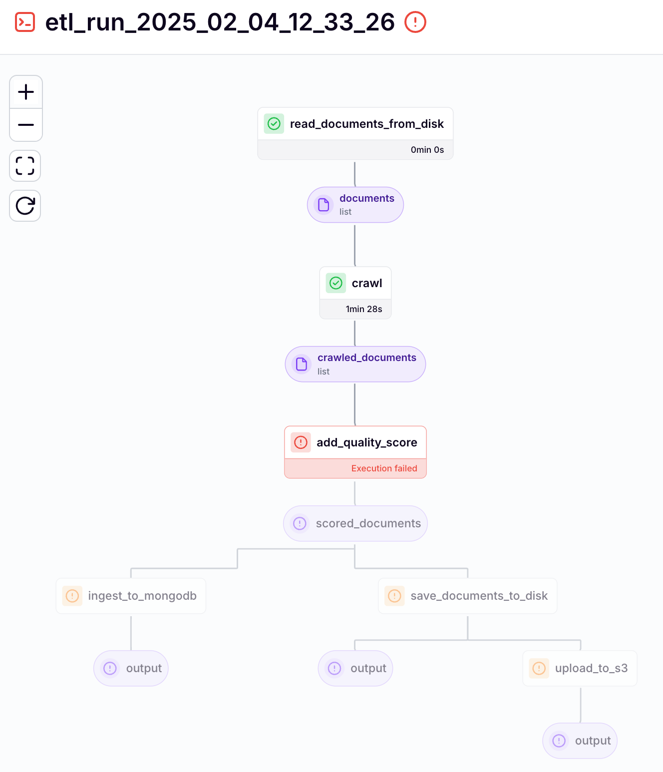
Ultimately, if we click on a specific pipeline run, we can see the whole Directed Acyclic Graph (DAG) with all its steps. If it fails, we can see the steps it failed at. Also, as seen in Figure 5, we can easily visualize and track the output of each step.
There is much more to ZenML. However, to avoid creating a section that sounds like documentation, we will highlight its other features while building our AI assistant.
As we said in the previous section, this course will start with the ETL data pipeline, which will use our precomputed Notion dataset. Hence, let’s implement it in ZenML.
What does our ETL data pipeline look like when implemented in ZenML?
The heart of our pipeline is the
etl()function, decorated with ZenML's@pipelinedecorator (found at pipelines/etl.py). This function orchestrates the entire data flow, accepting configuration parameters that control its behavior - from specifying data directories to controlling parallel processing and quality scoring settings:
@pipeline
def etl(
    data_dir: Path,
    load_collection_name: str,
    to_s3: bool = False,
    max_workers: int = 10,
    quality_agent_model_id: str = "gpt-4o-mini",
    quality_agent_mock: bool = True,
) -> None:
The pipeline's workflow begins by setting up the data paths. We establish two key directories: one for reading the raw Notion data and another for storing the processed results:
    notion_data_dir = data_dir / "notion"
    crawled_data_dir = data_dir / "crawled"
The primary data processing flow consists of three major steps. First, we read the documents from the disk. Then, we crawl every link found in each document. Next, we enhance the documents with quality scores:
    documents = read_documents_from_disk(
        data_directory=notion_data_dir, nesting_level=1
    )
    crawled_documents = crawl(documents=documents, max_workers=max_workers)
    enhanced_documents = add_quality_score(
        documents=crawled_documents,
        model_id=quality_agent_model_id,
        mock=quality_agent_mock,
        max_workers=max_workers,
    )
The final stage of our pipeline handles data persistence. We save the enhanced documents to disk, optionally upload them to S3, and finally load them into MongoDB for downstream processing:
    save_documents_to_disk(documents=enhanced_documents, output_dir=crawled_data_dir)
    if to_s3:
        upload_to_s3(
            folder_path=crawled_data_dir,
            s3_prefix="second_brain_course/crawled",
            after="save_documents_to_disk",
        )
    ingest_to_mongodb(
        models=enhanced_documents,
        collection_name=load_collection_name,
        clear_collection=True,
    )
In Figure 6, we can see what the ETL pipeline looks like in ZenML:

In future sections of the article, we will zoom in on each step and understand how it works.
One last key feature of ZenML is that it can be configured through YAML configuration files (one per pipeline). This allows you to easily configure each pipeline run without touching the code. Most importantly, you can track and version the configuration of each pipeline run, which is critical for reproducibility and debugging.
Let’s look at it in more detail (found under configs/etl.yaml):
parameters:
  data_dir: data/
  load_collection_name: raw
  to_s3: false
  max_workers: 4
  quality_agent_model_id: gpt-4o-mini
  quality_agent_mock: false
As you can see, it’s a YAML file that is one-on-one with the pipeline Python function parameters. As the pipeline function acts as the entry point to your application, it makes sense to be able to configure it from a clean YAML file that can be easily tracked by git instead of tweaking the values from the CLI.
If you are curious to learn more about ZenML, they have some fantastic guides while also learning production MLOps and LLMOps:
3. Exploring the collected Notion data
In Lesson 1, we explored how our data looks directly in Notion. However, as we start working with it only after our data collection pipeline collects it, we have to visualize how the data we ingest from S3 looks like, as that is what we will work with.
The data is stored in JSON, containing the content of the Notion document in Markdown, along with its metadata and embedded URLs. Here is one sample:
{
    "id": "8eb8a0ed6afffaa581ef6dff9b3eec17",
    "metadata": {
        "id": "8eb8a0ed6afffaa581ef6dff9b3eec17",
        "url": "https://www.notion.so/Training-Fine-tuning-LLMs-8eb8a0ed6afffaa581ef6dff9b3eec17",
        "title": "Training & Fine-tuning LLMs",
        "properties": {
            "Type": "Leaf"
        }
    },
    "parent_metadata": {
        "id": "6cfa25bcea00377355cfe21f7dfaadff",
        "url": "",
        "title": "",
        "properties": {}
    },
    "content": "# Resources [Community]\n\n\t<child_page>\n\t# Number of samples for fine-tuning based on general, domain, task-specific
... # The rest of the document in Markdown format
"
    "content_quality_score": null,
    "summary": null,
    "child_urls": [
        "https://github.com/huggingface/trl/",
        "https://www.linkedin.com/company/liquid-ai-inc/",
        "https://github.com/unslothai/unsloth/",
        "https://arxiv.org/abs/2106.09685/",
        "https://paperswithcode.com/sota/code-generation-on-humaneval/",
        "https://github.com/axolotl-ai-cloud/axolotl/",
        "https://neptune.ai/blog/llm-fine-tuning-and-model-selection-with-neptune-transformers/",
        "https://arxiv.org/abs/2305.14314/"
}
Every document is stored in its own JSON following the same structure:
metadata: containing the source URL plus other details about the source
parent_metadata: containing the parent’s URL, plus other details about the parent (if empty, it has no parent)
content: the actual content in Markdown format
child_urls:
The next step is to load this data into Python while ensuring that each JSON file is valid (has the expected structure and data types). The preferred method for this is using Pydantic.
How do we model this data into a Pydantic class?
Let’s see how we can model our data using Pydantic, the go-to Python package for defining modern data structures in Python. But first, let’s make a quick analogy to LangChain.
When working with LangChain, one of the fundamental building blocks is the Document class. Let's explore how we can implement our own version that builds upon LangChain's concept while respecting our custom functionality and needs.
Our
Documentclass maintains LangChain's core principle of combining content with metadata while extending it with additional features. Each document has its unique identifier, content, and structured metadata, plus we've added support for document hierarchies, quality assessment, and summarization.
class Document(BaseModel):
    id: str = Field(default_factory=lambda: utils.generate_random_hex(length=32))
    metadata: DocumentMetadata
    parent_metadata: DocumentMetadata | None = None
    content: str
    content_quality_score: float | None = None
    summary: str | None = None
    child_urls: list[str] = Field(default_factory=list)

    @classmethod
    def from_file(cls, file_path: Path) -> "Document":
        json_data = file_path.read_text(encoding="utf-8")
        return cls.model_validate_json(json_data)

    def __eq__(self, other: object) -> bool:
        if not isinstance(other, Document):
            return False
        return self.id == other.id

    def __hash__(self) -> int:
        return hash(self.id)
While LangChain uses a simple dictionary for metadata, we've created a dedicated
DocumentMetadataclass. This structured approach ensures consistent metadata across our pipeline and provides better type safety:
class DocumentMetadata(BaseModel):
    id: str
    url: str
    title: str
    properties: dict
By storing the source URL and the parent’s source URL within the metadata while doing RAG, we can show the user the source used as context and where the source originates from. For example, we can show the user from which Notion database the link was accessed and what link was crawled.
One last thing to highlight is that storing the parent_metadata and child_urls fields can extend this to multi-hoping algorithms simulating a GraphDB structure. We won’t do that in our course, but it’s good to know that you don’t necessarily need a GraphDB to do GraphRAG. In cases where you need parents or children from only 2-3 levels relative to your data point, modeling your data using relationships is good enough to get started.
Before we discuss the implementation, we need to review some basic requirements for crawling.
4. Looking into requirements for crawling
So, how does crawling work? Essentially, it's about automatically visiting web pages, extracting the content, and following links to discover more pages. This process can be very complex because every website has a different structure, and there are many ways to present content. You'll need to ensure you're able to handle this complexity.
Before crawling any website, you must check the site’s crawling limitations. You can do that by adding /robots.txt to the end of the website's URL. This file tells you which parts of the website are off-limits for web crawlers. Respecting these rules is essential since they protect the website from overloading and ensure you’re not crawling sensitive information.

Now, if you want to crawl a website, you’ll also need to know all the pages you need to visit. You might think you can start from a home page and follow all the links. However, you'll soon discover this approach can be inefficient and may not capture all website pages.
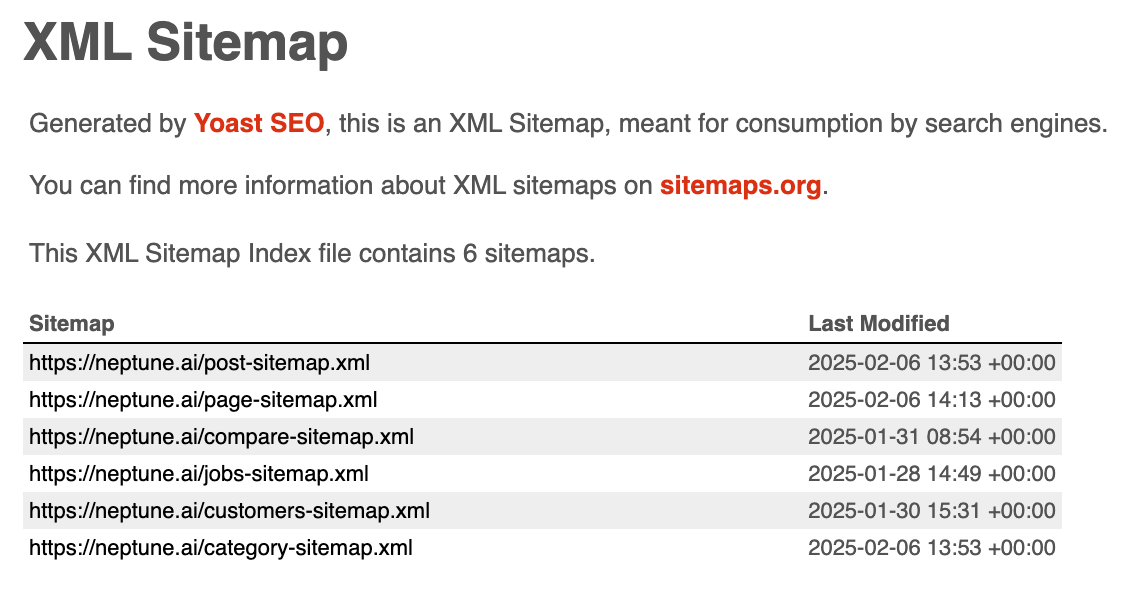
That’s why many websites provide a sitemap that lists all their pages. The sitemap is usually added to better index the site for search engines (which also crawl it), but we can also leverage it to get a list of recurrent links we can crawl easily.
You can usually find this sitemap by adding /sitemap.xml to the end of the website's URL. This file gives you a structured list of all the website’s sub-URLs, which makes it a lot easier to do a recursive crawl, which means you can follow all the links on the website.
Now, you need a tool to do all this.
We will use Crawl4AI for crawling, an open-source web crawling framework specifically designed to scrape websites and format the output for LLMs to understand.
The tool has built-in HTML to Markdown conversion, which is perfect for our needs. Crawl4AI is designed to be efficient, fast, and easy to set up. It can handle things like proxies, session management, and removing irrelevant content, which are not easy to handle.
5. Implementing crawling
How can we apply these principles to our crawling algorithm?
Our code is educative and harmless. Hence, to keep things simple, we will skip checking the robots.txt file. But it’s super important to remember this when working with real-world products.
Also, to avoid working with too many links, we will skip checking the sitemap.xml file and stick to the links found directly on our Notion pages. However, we could easily augment our dataset by accessing the sitemap.xml file of each link we use from Notion, expanding our dataset exponentially.
With that in mind, let’s dig into the implementation.
At the heart of our crawling step, we have a ZenML step that orchestrates the crawling process (which is called from the ZenML pipeline):
@step
def crawl(
    documents: list[Document], max_workers: int = 10
) -> Annotated[list[Document], "crawled_documents"]:
    crawler = Crawl4AICrawler(max_concurrent_requests=max_workers)
    child_pages = crawler(documents)

    augmented_pages = documents.copy()
    augmented_pages.extend(child_pages)
    augmented_pages = list(set(augmented_pages))
To track our crawling progress and provide insights into the pipeline's performance, we add metadata about the number of documents processed:
    step_context = get_step_context()
    step_context.add_output_metadata(
        output_name="crawled_documents",
        metadata={
            "len_documents_before_crawling": len(documents),
            "len_documents_after_crawling": len(augmented_pages),
            "len_documents_new": len(augmented_pages) - len(documents),
        },
    )

    return augmented_pages
This metadata is attached to the crawled_documents output artifact and can be visualized from ZenML’s dashboard. As shown in Figure 9, it helps us monitor and debug each pipeline run.

Now, let's look at our Crawl4AICrawler class implementation, which leverages the powerful features of Crawl4AI. This crawler is designed to handle concurrent web crawling efficiently while providing clean, LLM-ready output in Markdown format.
The crawler class under the hood uses Crawl4AI's AsyncWebCrawler with its sophisticated browser and crawler configurations. As the class is called from the ZenML step, which runs in a Python synchronous process, and the crawler uses an async method, we must define and manage an async loop internally. Using async, it’s a powerful mechanism in Python to manage concurrently I/O dependent processes such as crawling or API requests:
class Crawl4AICrawler:
    def __init__(self, max_concurrent_requests: int = 10) -> None:
        self.max_concurrent_requests = max_concurrent_requests

    def __call__(self, pages: list[Document]) -> list[Document]:
        try:
            loop = asyncio.get_running_loop()
        except RuntimeError:
            return asyncio.run(self.__crawl_batch(pages))
        else:
            return loop.run_until_complete(self.__crawl_batch(pages))
The core crawling logic happens in the
__crawl_batchmethod. We use Crawl4AI'sCacheMode.BYPASSto ensure fresh content:
    async def __crawl_batch(self, pages: list[Document]) -> list[Document]:
        process = psutil.Process(os.getpid())
        start_mem = process.memory_info().rss

        semaphore = asyncio.Semaphore(self.max_concurrent_requests)
        all_results = []

        async with AsyncWebCrawler(cache_mode=CacheMode.BYPASS) as crawler:
            for page in pages:
                tasks = [
                    self.__crawl_url(crawler, page, url, semaphore)
                    for url in page.child_urls
                ]
                results = await asyncio.gather(*tasks)
                all_results.extend(results)

        successful_results = [result for result in all_results if result is not None]
Finally, each URL is processed by the
__crawl_urlmethod, which utilizes Crawl4AI's powerful content extraction and Markdown generation capabilities. As we kick off all the jobs simultaneously, we control how many concurrent requests we can run simultaneously using thesemaphorePython object. This is useful for managing your computer’s resources or API limits:
    async def __crawl_url(
        self,
        crawler: AsyncWebCrawler,
        page: Document,
        url: str,
        semaphore: asyncio.Semaphore,
    ) -> Document | None:
        async with semaphore:
            result = await crawler.arun(url=url)
            await asyncio.sleep(0.5)  # Rate limiting

            if not result or not result.success or result.markdown is None:
                return None

            child_links = [
                link["href"]
                for link in result.links["internal"] + result.links["external"]
            ]
            title = result.metadata.pop("title", "") if result.metadata else ""

            return Document(
                id=utils.generate_random_hex(length=32),
                metadata=DocumentMetadata(
                    id=document_id,
                    url=url,
                    title=title,
                    properties=result.metadata or {},
                ),
                parent_metadata=page.metadata,
                content=str(result.markdown),
                child_urls=child_links,
            )
Crawl4AI is particularly well-suited for our needs as it's designed to be LLM-friendly. It generates clean Markdown output directly and handles all the formatting complexity behind the scenes.
The next step from our ETL pipeline is to compute the quality score.
6. Computing the quality score
Assessing content quality is crucial when processing documents in data pipelines. RAG systems can be incredibly powerful as long they use high-quality context. Also, when it comes to fine-tuning LLMs, using high-quality samples is the most critical aspect in which you should invest.
Thus, let's explore a sophisticated two-stage system that combines quick heuristic rules with an advanced LLM-based evaluation approach.
As parsing the document using an LLM can quickly increase the latency and costs of your system, we try first to do our best and compute the quality score using a set of heuristics. The key is to use heuristics where we are 100% sure we can score the documents. Next, for more complex and nuanced scenarios, we use the LLM.
Our ZenML pipeline step orchestrates the quality scoring process, starting with fast heuristics and falling back to the LLM-based method when needed:
@step
def add_quality_score(
    documents: list[Document],
    model_id: str = "gpt-4o-mini",
    mock: bool = False,
    max_workers: int = 10,
) -> Annotated[list[Document], "scored_documents"]:
    heuristic_quality_agent = HeuristicQualityAgent()
    scored_documents: list[Document] = heuristic_quality_agent(documents)

    scored_documents_with_heuristics = [
        d for d in scored_documents if d.content_quality_score is not None
    ]
    documents_without_scores = [
        d for d in scored_documents if d.content_quality_score is None
    ]

    quality_agent = QualityScoreAgent(
        model_id=model_id, mock=mock, max_concurrent_requests=max_workers
    )
    scored_documents_with_agents: list[Document] = quality_agent(
        documents_without_scores
    )
The heuristic agent provides a quick first pass by analyzing URL density - a simple yet effective way to filter out low-quality documents that are mostly just collections of links:
class HeuristicQualityAgent:
    def __call__(self, documents: list[Document]) -> list[Document]:
        ...

    def __score_document(self, document: Document) -> Document:
        if len(document.content) == 0:
            return document.add_quality_score(score=0.0)

        url_based_content = sum(len(url) for url in document.child_urls)
        url_content_ratio = url_based_content / len(document.content)

        if url_content_ratio >= 0.7:
            return document.add_quality_score(score=0.0)
        elif url_content_ratio >= 0.5:
            return document.add_quality_score(score=0.2)
        return document
For more nuanced evaluation, we define a structured response format to ensure consistent scoring from our LLM:
class QualityScoreAgent:
    SYSTEM_PROMPT_TEMPLATE = """You are an expert judge tasked with evaluating the quality of a given DOCUMENT.

Guidelines:
1. Evaluate the DOCUMENT based on generally accepted facts and reliable information.
2. Evaluate that the DOCUMENT contains relevant information and not only links or error messages.
3. Check that the DOCUMENT doesn't oversimplify or generalize information in a way that changes its meaning or accuracy.

Analyze the text thoroughly and assign a quality score between 0 and 1, where:
- **0.0**: The DOCUMENT is completely irrelevant containing only noise such as links or error messages
- **0.1 - 0.7**: The DOCUMENT is partially relevant containing some relevant information checking partially guidelines
- **0.8 - 1.0**: The DOCUMENT is entirely relevant containing all relevant information following the guidelines

It is crucial that you return only the score in the following JSON format:
{{
    "score": <your score between 0.0 and 1.0>
}}

DOCUMENT:
{document}
"""
The
QualityScoreAgentimplements sophisticated batch processing with concurrency control and rate limiting (similar to what you have seen in the crawler class). Calling OpenAI’s API in batch mode can quickly hit its request limits. To find a balance between process time and successfully scoring each document, we first called the API for each document using a shorter wait time between API calls. Next, for each API request that failed, we retry it with a longer wait period:
    async def __get_quality_score_batch(
        self, documents: list[Document]
    ) -> list[Document]:
        scored_documents = await self.__process_batch(documents, await_time_seconds=7)
        documents_with_scores = [
            doc for doc in scored_documents if doc.content_quality_score is not None
        ]
        documents_without_scores = [
            doc for doc in scored_documents if doc.content_quality_score is None
        ]

        # Retry failed documents with increased await time
        if documents_without_scores:
            retry_results = await self.__process_batch(
                documents_without_scores, await_time_seconds=20
            )
            documents_with_scores += retry_results

        return scored_documents
For each document, we format the input prompt, make the API request, and wait for a given period to avoid API request limits:
    async def __get_quality_score(
        self,
        document: Document,
        semaphore: asyncio.Semaphore | None = None,
        await_time_seconds: int = 2,
    ) -> Document | None:
        async def process_document() -> Document:
            input_user_prompt = self.SYSTEM_PROMPT_TEMPLATE.format(
                document=document.content
            )

            response = await acompletion(
                model=self.model_id,
                messages=[
                    {"role": "user", "content": input_user_prompt},
                ],
                stream=False,
            )
            await asyncio.sleep(await_time_seconds)  # Rate limiting

            raw_answer = response.choices[0].message.content
            quality_score = self._parse_model_output(raw_answer)
            return document.add_quality_score(score=quality_score.score)
The last step is to check that the LLM’s output follows our desired format by leveraging a Pydantic class:
class QualityScoreResponseFormat(BaseModel):
    """Format for quality score responses from the language model.

    Attributes:
        score: A float between 0.0 and 1.0 representing the quality score.
    """

    score: float


def _parse_model_output(
        self, answer: str | None
    ) -> QualityScoreResponseFormat | None:
        if not answer:
            return None

        try:
            dict_content = json.loads(answer)
            return QualityScoreResponseFormat(
                score=dict_content["score"],
            )
        except Exception:
            return None
Here are two important observations we still have to point out:
Instead of directly using OpenAI’s API, we used litellm, a wrapper over multiple popular LLM APIs, such as OpenAI, Antrophic, Cohere, and more. We recommend using them, as they allow you to experiment easily with various providers without touching the code.
To further optimize the system by reducing costs and the chance of request-limit errors, you can use OpenAI’s batch API. In this way, you can send multiple documents per request.
The last step is to see how we can load the processed documents to MongoDB.
7. Loading the standardized data to a document database
When building data pipelines, you often need a reliable way to store and retrieve your processed documents. This type of storage is often known as the data warehouse.
In our use case, out of simplicity, we used MongoDB, which is not a data warehouse by the book, but for text data, it gets the job done well.
We implemented the MongoDBService class to interact with MongoDB. This class provides a generic interface for handling any Python structure that follows a Pydantic model structure.
The class is designed to be flexible, using Python's generic typing to work with any Pydantic model. This means you can use it to store different types of Python data structures while maintaining type safety and validation:
T = TypeVar("T", bound=BaseModel)

class MongoDBService(Generic[T]):
    def __init__(
        self,
        model: Type[T],
        collection_name: str,
        database_name: str = settings.MONGODB_DATABASE_NAME,
        mongodb_uri: str = settings.MONGODB_URI,
    ) -> None:
The
ingest_documents()method is where the magic happens. It takes your Pydantic models and safely stores them in MongoDB. The method includes validation and proper error handling to ensure your data is stored correctly:
    def ingest_documents(self, documents: list[T]) -> None:
        try:
            if not documents or not all(
                isinstance(doc, BaseModel) for doc in documents
            ):
                raise ValueError("Documents must be a list of Pycantic models.")

            dict_documents = [doc.model_dump() for doc in documents]

            # Remove '_id' fields to avoid duplicate key errors
            for doc in dict_documents:
                doc.pop("_id", None)

            self.collection.insert_many(dict_documents)
            logger.debug(f"Inserted {len(documents)} documents into MongoDB.")
        except errors.PyMongoError as e:
            logger.error(f"Error inserting documents: {e}")
            raise
That’s it. We are finally done implementing our data pipeline.
The last step is to look at how we can run the code.
8. Running the code
The best way to set up and run the code is through our GitHub repository, where we have documented everything you need. We will keep these instructions only in our GitHub to avoid having the documentation scattered throughout too many places (which is a pain to maintain and use).
But to give a sense of the “complexity” of running the code, you have to run ONLY the following commands using Make:
make local-infrastructure-up    # 1. Spin up the infrastructure
make download-notion-dataset    # 2. Download the Notion dataset
make etl-pipeline               # 3. Run the ETL pipeline through ZenML
That’s all it takes to crawl and compute the quality score for all the documents.
While the ETL pipeline is running, you can visualize it on ZenML’s dashboard by typing in your browser: http://127.0.0.1:8237
Conclusion
This lesson taught you what it takes to build the data pipelines to implement a Second Brain AI assistant.
We walked you through the architecture of the data pipelines, how to manage them with an MLOps framework such as ZenML, what the Notion data looks like, and what you should consider when crawling.
We learned how to crawl custom links at scale using Crawl4AI, compute a quality score for all your documents using heuristics and LLMs, and create a snapshot of the data in MongoDB.
Lesson 3 will teach you how to generate a high-quality summarization instruction dataset using distillation and how to load it to Hugging Face.
💻 Explore all the lessons and the code in our freely available GitHub repository.
If you have questions or need clarification, feel free to ask. See you in the next session!
Whenever you’re ready, there are 3 ways we can help you:
Perks: Exclusive discounts on our recommended learning resources
(live courses, self-paced courses, learning platforms and books).
The LLM Engineer’s Handbook: Our bestseller book on teaching you an end-to-end framework for building production-ready LLM and RAG applications, from data collection to deployment (get up to 20% off using our discount code).
Free open-source courses: Master production AI with our end-to-end open-source courses, which reflect real-world AI projects, covering everything from system architecture to data collection and deployment.
References
Decodingml. (n.d.). GitHub - decodingml/second-brain-ai-assistant-course. GitHub. https://github.com/decodingml/second-brain-ai-assistant-course
MongoDB: the Developer Data platform. (n.d.). MongoDB. https://www.mongodb.com
Pydantic. (n.d.). GitHub - pydantic/pydantic: Data validation using Python type hints. GitHub. https://github.com/pydantic/pydantic
Unclecode. (n.d.). GitHub - unclecode/crawl4ai: 🚀🤖 Crawl4AI: Open-source LLM Friendly Web Crawler & Scraper. GitHub. https://github.com/unclecode/crawl4ai
ZenML - MLOps framework for infrastructure agnostic ML pipelines. (n.d.). https://zenml.io
Cole Medin. (2025, January 13). Turn ANY Website into LLM Knowledge in SECONDS [Video]. YouTube. https://www.youtube.com/watch?v=JWfNLF_g_V0
Sponsors
Thank our sponsors for supporting our work — this course is free because of them!


Images
If not otherwise stated, all images are created by the author.
Subject: Issue Accessing notion/notion.zip in decodingml-public-data S3 Bucket
Dear Decoding ML Team,
I have spent a week part time trying to follow the instruction of part2. I have purchased a Claude subscription to help and exhaust each day. Ditto Grok. Gemini allows me more tokens and I have spent many hours trying to get it to work. I asked gemini to script me a key question to you which is as follows (I am not sure it gets to the root of the issue but I have been meticulous in following instruction including following Claude/grok/gemini advice, which frankly is very impressive but I have done some things 12 times in circular loops - I am seriously doubting it is worthwhile continuing although I am extremely appreciative of what you are offering especially for free (though it has "cost" me a deal in time). Anyways here is the AI generated question....
I'm currently working through the "Second Brain Offline" course and have encountered an issue when attempting to download the notion/notion.zip file from the decodingml-public-data S3 bucket.
Specifically, I'm receiving a 403 Forbidden error despite using the --no-sign-request flag in the command:
Bash
python second-brain-offline/src/tools/use_s3.py download decodingml-public-data notion/notion.zip data/notion --no-sign-request
This error indicates that the bucket or the object may not be configured for public read access.
Given that the course materials do not explicitly require AWS credentials (focusing primarily on Hugging Face Inference Endpoints), I believe this is likely a configuration issue with the bucket's permissions.
Could you please:
Verify the permissions of the decodingml-public-data bucket and the notion/notion.zip object to ensure they allow public read access?
Provide an alternative download method for the notion/notion.zip file if public access is not intended?
Thank you for your prompt attention to this matter. I'm eager to continue progressing through the course.
Sincerely,
John
Thank you very much!
I'm also working on a project to track project releases and want to implement RAG (Retrieval-Augmented Generation) to easily retrieve release details. I believe this course will be very helpful for my project.