A journey where you will have the chance to learn to implement an LLM application using agents, advanced Retrieval-augmented generation (RAG), fine-tuning, LLMOps, and AI systems techniques.
Using general-purpose large language models (LLMs) to build GenAI apps from APIs, such as OpenAI, Antrophic, or Google, is great until it isn’t.
Building your LLM and RAG application around these providers is a solid start to create a PoC or MVP quickly, but you will soon realize that:
Your API bill is skyrocketing.
You are vendor-locked in, and your application’s performance can degrade anytime (as you don’t have control over the LLMs).
You don’t have control over your data.
Thus, you need to find ways to optimize costs and gain more control over your models and data.
That’s why the next natural step is learning to use open-source LLMs (e.g., Llama, Qwen, or DeepSeek) to power your GenAI applications. Using swarms of open-source smaller language models (SLM) specialized in specific tasks is a solid strategy in reducing costs and gaining control over your AI system.
Thus, when using open-source models, you have two options:
Use them as they are and deploy them on your cloud provider of choice (e.g., AWS Bedrock, Hugging Face Dedicated Endpoints, Modal, on-prem)
If the models are too inaccurate for your use case, you must first fine-tune them on your specific task or domain (using Hugging Face’s TRL and Unsloth) and then deploy them.
In this lesson, we will assume that you need to do both. Therefore, using the summarization instruction dataset from Lesson 3, we will fine-tune a small language model (SLM) specialized in summarizing web documents collected from the internet.
Then, we will deploy it to Hugging Face’s Inference Endpoints serverless service and use it to summarize documents within our application.
To conclude, while implementing the training pipeline, we will learn the following:
When and how to fine-tune open-source LLMs using LoRA and QLoRA.
Using TRL, Unsloth, and Comet to fine-tune LLMs efficiently.
Architecting modular and scalable training pipelines with MLOps and production in mind.
Evaluating the fine-tuned LLM using vLLM.
Deploying the fine-tuned LLM as a real-time API endpoint to Hugging Face Inference Endpoints.
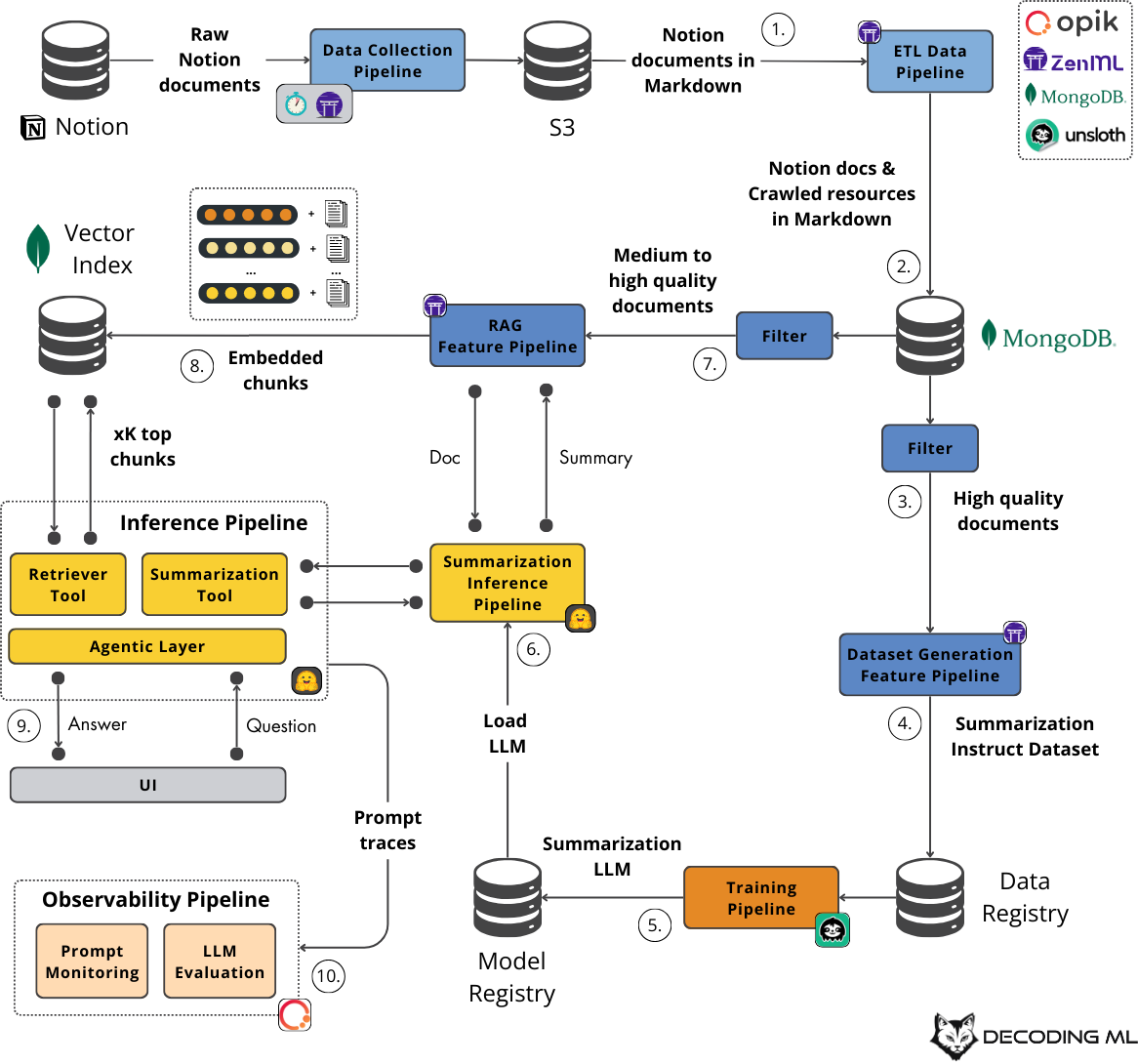
Figure 1: The architecture of the Second Brain AI assistant powered by RAG, LLMs and agents (what is built during the 6-lesson course).
Let’s get started. Enjoy!
Podcast version of the lesson
1×
0:00
-16:17
Table of contents:
Prompt engineering vs. RAG vs. Fine-tuning: When to fine-tune?
Understanding how LLMs are trained
Fine-tuning with distillation
Exploring LoRA and QLoRA fine-tuning techniques
Choosing our fine-tuning toolbelt
Architecting the training pipeline
Fine-tuning open-source LLMs
Loading the fine-tuned LLM into a model registry
Running the fine-tuned LLM from the model registry
Evaluating the fine-tuned LLM
Deploying the fine-tuned LLM as a real-time API endpoint
Running the code
1. Prompt engineering vs. RAG vs. Fine-tuning: When to fine-tune?
Fine-tuning is costly as it involves gathering data, generating the instruction dataset, training the model, storing it, deploying it, and maintaining it.
Thus, your first job is determining whether you can finish the task without fine-tuning it.
In Figure 2, you can visualize a standard roadmap determining whether fine-tuning is necessary. You should always ask yourself the following questions:
Is prompt engineering enough? (e.g., few-shot learning)
Is prompt engineering + RAG enough?
You should continue fine-tuning an LLM only if you cannot finish the job with prompt engineering and RAG.
Figure 2: Prompt engineering vs. RAG vs. Fine-tuning: When to fine-tune an LLM? (Image inspired by Maxime Labonne’s section of the LLM Engineer’s Handbook)
Note how critical evaluation is regardless of what technique you adopt in improving the outputs of the LLM. That’s why, in reality, your first job is to build an end-to-end system that you can evaluate. Only at that point in your project’s maturity should you consider prompt engineering vs. RAG vs. fine-tuning.
We want to create a small language model (SLM) specialized in summarizing web documents without complicated prompt engineering techniques (we have an SLM with a small context window) to increase accuracy. Therefore, we assume that we have to fine-tune the LLM.
With that in mind, let’s dig into the LLM fine-tuning world.
2. Understanding how LLMs are trained
LLMs like the ones powering your AI assistant go through several training phases. Each phase builds on the previous one, gradually transforming raw text data into a helpful assistant to understand and respond to your needs.
The journey begins with pretraining for completion. During this phase, the model learns to predict what comes next in a sequence of text by processing massive amounts of data from the internet - we're talking trillions of tokens, equivalent to millions of books. The model develops a statistical understanding of language patterns, learning which words will likely follow others in different contexts. For example, if you write "My favorite color is," the model learns that words like "blue" or "green" are more likely to follow than "car" or "pizza."
This pretraining phase is incredibly resource-intensive, consuming about 98% of the overall compute and data resources needed to create a model like ChatGPT. The resulting pretrained model has absorbed enormous knowledge but doesn't yet know how to be helpful or follow instructions.
That's where supervised fine-tuning (SFT) comes in. During this phase, the model is shown examples of how to respond to different types of prompts appropriately. These examples follow a format of (prompt, response) pairs created by highly educated human labelers or other powerful LLMs (a process known as distillation — what we are doing in this course).
For instance, if the prompt is "How to make pizza?", the model learns that it should provide a helpful answer rather than just continuing the question or adding context.
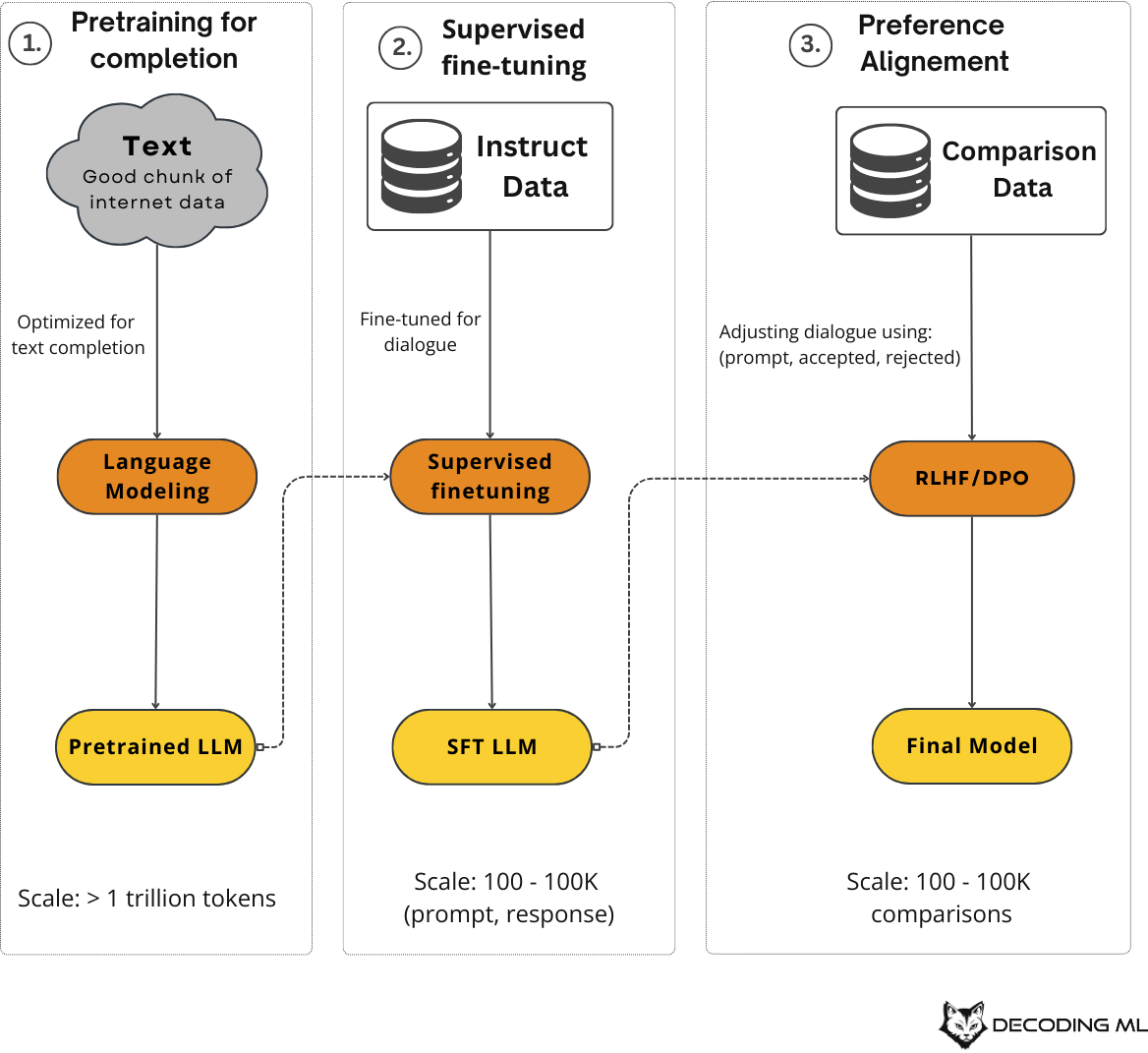
Figure 3: The 3 main stages of training an LLM
The final phase is preference alignment, where we further fine-tune the model using comparison pairs (prompt, accepted, rejected) that guide the model in what style to respond to specific prompts. This increases the probability that prompt X should respond in way Y instead of way Z.
This preference alignment phase is the final polish that transforms a model that can follow instructions into one that tries to provide the most helpful and appropriate responses possible.
Through these three phases—pretraining for completion, supervised fine-tuning, and preference alignment—raw text data is transformed into the sophisticated AI assistants we interact with today.
But how does fine-tuning with distillation (the technique we will adopt in this lesson) fit into all of this? Let’s dig into that.
3. Fine-tuning with distillation
To create our LLM, which specializes in summarizing web documents, we will focus only on supervised fine-tuning (SFT).
More concretely, we will take a pretrained model, such as Llama 8B 3.1, and further fine-tune it on the instruction dataset generated in Lesson 3.
As the dataset was generated by a more powerful model, such as gpt-4o (not Llama 8B 3.1), this process is known as fine-tuning with distillation. To rephrase it, we use a powerful model to generate the fine-tuning dataset, which we use to fine-tune a smaller model. Intuitively, we distill the knowledge from the more powerful model to the smaller one through the dataset.
This process is usually used in teacher-student distillation techniques, where both models are used during training. Here, we use the teacher model only during dataset generation. This method has proved productive in the generative AI world.
Figure 4: Where does fine-tuning with distillation fit in creating our specialized LLM in summarization?
We can also adopt a similar technique for the preference alignment step to generate a comparison dataset and use strategies such as RLHF and DPO to align the model further. Although this is out of the scope of this lesson, it would be a helpful exercise for you to implement it yourself.
Now that we understand how LLMs are fine-tuned and where fine-tuning with distillation fits the bigger picture, we must cover the LoRA and QLoRA fine-tuning techniques we will use during SFT.
4. Exploring LoRA and QLoRA fine-tuning techniques
You have three main approaches when fine-tuning LLMs: full fine-tuning, LoRA, and QLoRA. Each has its own strengths and trade-offs that make it suitable for different scenarios.
Full fine-tuning is the most straightforward approach - you retrain every parameter in the base model. While this often gives the best results, it's highly resource-intensive. For a 7B parameter model using 32-bit precision, you'd need about 112GB of VRAM, and a 70B model would require a staggering 1,120 GB VRAM. This is because each parameter needs memory for the parameter itself, its gradient, and optimizer states.
The memory formula during training looks like this: `Parameters + Activations + Gradients + Optimizer States`.
With standard settings, this translates to about 16 bytes per parameter, making full fine-tuning impractical without specialized hardware. Additionally, full fine-tuning directly changes the pre-trained weights, risking "catastrophic forgetting," where the model loses previously learned knowledge.
LoRA(Low-Rank Adaptation) offers a clever solution to these challenges. Instead of modifying the original weight matrix W, LoRA introduces two smaller matrices, A and B, that form a low-rank update. The effective weight becomes W' = W + BA, where W remains frozen and only A and B are trained. This dramatically reduces memory usage and training time while preserving the knowledge of the pre-trained model.
The key hyperparameters for LoRA include the rank (r), which determines the size of the matrices (typically starting at r=8, but values up to 256 can work well), and alpha (α), a scaling factor applied to the update. You can also add dropout (usually 0-0.1) to prevent overfitting.
LoRA can be applied to various model components - initially just the query (Q) and value (V) matrices in attention layers, but now commonly extended to key (K) matrices, output projections, feed-forward blocks, and linear output layers. With LoRA, you can fine-tune a 7B parameter model on a single GPU with just 14-18GB of VRAM. For example, when targeting all modules with rank 16, a Llama 3 8B model only trains 42 million parameters (about 0.52% of the total).
Figure 5: Full fine-tuning vs. LoRA vs. QLoRA (Section and image inspired by Maxime Labonne’s section of the LLM Engineer’s Handbook)
QLoRA improves memory efficiency even further by combining LoRA with quantization. It quantizes the base model to a custom 4-bit format called NormalFloat (NF4), significantly reducing memory requirements. To manage memory spikes, QLoRA also employs double quantization (quantizing the quantization constants themselves) and paged optimizers.
The memory savings are substantial - for a 7B model, QLoRA reduces peak memory usage from 14GB to 9.1GB during initialization (35% reduction) and from 15.6GB to 9.3GB during fine-tuning (40% reduction). This comes at the cost of slower training - QLoRA is about 30% slower than LoRA - but the model performance remains comparable.
When deciding between these techniques, consider your resources and priorities. If you have limited GPU memory or want to fine-tune very large models, QLoRA is your best bet. If training speed matters more and you have sufficient memory, LoRA offers a good balance. Full fine-tuning should be reserved for cases where you have abundant computational resources and need the absolute best performance.
We'll use LoRA with Unsloth to balance efficiency and performance for our document summarization task. This makes the fine-tuning process available on accessible hardware, such as what you find on Google Colab (e.g., L4 Nvidia GPU).
But, as L4 Nvidia GPU is available only to Colab paid users, we will offer the possibility to use QLoRA, which works on T4 Nvidia GPUs, available for free on Google Colab.
The last step before implementation is to examine our tool choice and understand how everything fits together in the training pipeline architecture.
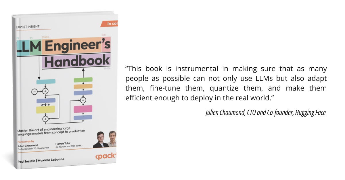
The fine-tuning sections were inspired by Maxime Labonne, the co-author of the LLM Engineer’s Handbook. To read more on anything related from sections 1 to 5, consider supporting us by buying our book:
We will fine-tune our summarization LLM using mainly 3 tools:
TRL: Hugging Face created and maintained this library to train LLMs using SFT and preference alignment. It is a popular library that tends to be the most up-to-date regarding algorithms.
Unsloth: Created by Daniel and Michael Han, Unsloth speeds up training (2x) and cuts VRAM use (up to 80%) with custom kernels. Based on TRL, it supports GGUF quantization for running fine-tuned models in Ollama and llama.cpp. Unsloth also collaborates with Meta, Google, and Microsoft to fix bugs in open models like Llama, making it an excellent choice for accurate open-source AI.
Comet: A popular experiment tracker that allows you to track, manage, and compare your fine-tuning experiments. Using an experiment tracker, you can easily visualize and reproduce the results of your training (see an example)
For example, we will fine-tune a Llama 3.1 8B LLM in our use case. Using Unsloth for fine-tuning reduced the VRAM usage by 70%, allowing us to do a full fine-tuning on lower-end hardware, such as T4/L4 Nvidia GPUs.
Less memory usage and faster training times mean lower costs, more accessibility, experiments, and innovation. That’s why Unsloth is making waves in the LLM community, already having 30k+ stars on GitHub.
Depending on the LLM of choice and training techniques, a custom kernel can reduce memory usage by 50% and 80%. However, for most use cases, a ~70% reduction in memory is expected.
When architecting an ML component (or any software component), starting with its interface is good practice. In our case, the training pipeline will do the following:
Have as input the training features (aka the dataset) from the Hugging Face data registry and the base model from the Hugging Face model registry.
Have as output the fine-tuned LLM (specialized in summarizing web documents) loaded into the Hugging Face model registry.
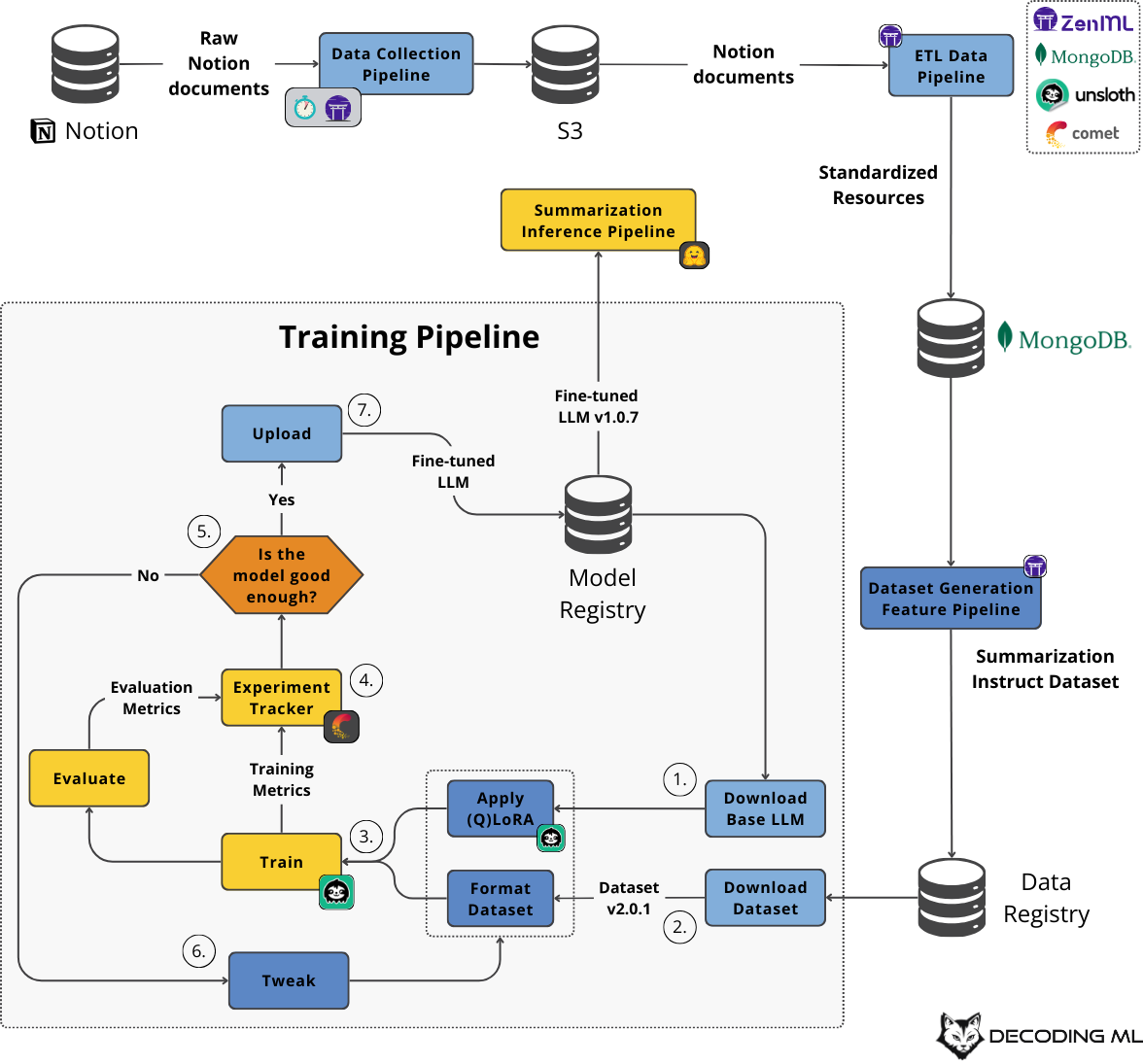
Figure 6: The architecture of the training pipeline relative to the rest of the Second Brain AI assistant components
Now that we’ve understood its interface, let’s take a deeper look at all the steps the training pipeline has to go through:
Download the base LLM (in our use case Llama 8B 3.1 Instruct) and apply the LoRA (or QLoRA) adapters
Download our custom summarization instruction dataset generated in Lesson 3 and format it into the correct format using an Alpaca template.
Using the base LLM and instruction dataset, we use Unsloth to fine-tune the LLM and specialize it into creating high-quality summaries for web documents.
Meanwhile, we evaluate the fine-tuned LLM and log the training and evaluation metrics into the Comet ML experiment tracker (here is an example).
The experiment tracker makes it easy to visualize and compare all the necessary metrics to decide whether the model is good enough.
If it’s not good enough, we tweak different hyperameters or data preprocessing methods and repeat steps 3 to 5.
If it’s good enough, we will upload it to the model registry, where we can deploy it as a real-time inference endpoint (here is our fine-tuned model).
Where is the training pipeline running?
The training pipeline is often within the scope of data scientists/AI researchers. Fully automating (as we did so far with the rest of the offline ML pipelines using ZenML) is not always good practice or even required.
The training pipeline is connected to the rest of the system through the data and model registries, so we can easily detach it from the rest of the AI system. Thus, we implemented it in Jupyter Notebooks, which allows us to provide more flexibility in research time.
Allowing the researchers to do their work in Jupyter Notebooks provides the following advantages:
Instead of connecting to cloud resources through SSH, they have a friendly GUI where they can do their work, removing friction.
Researchers are usually more used to using Jupyter Notebooks than SSH + Python scripts.
As a byproduct, they can experiment and innovate.
As a byproduct, they can easily visualize their data.
In our particular use case, we used Google Colab, which offers a freemium tier with access to T4 GPUs, which is perfect for our use case.
However, following a similar strategy, you can easily host the Jupyter Notebooks on your on-prem infrastructure or run them on any other cloud provider (AWS, Databricks, Azure, Lambda Labs, etc.).
How can we automate the training pipeline?
From our current state, we are not that far from implementing continuous training (CT). As the training pipeline is already connected with the rest of the system through the data and model registries, we just need a way to deploy our training pipeline code on an infrastructure that can run on a trigger.
The good news is that we already have ZenML, which is the perfect tool. Thus, instead of running the code manually from a Notebook, we deploy it to a cloud provider (e.g., AWS) and manage it through ZenML as the rest of the offline ML pipeline.
The only difference between the training and feature pipelines is that the former requires more computing power, takes longer to run, and is probably more costly. That’s why it’s common to keep the training pipeline a manual process and run it only when necessary.
With that in mind, we laid down all the foundations for understanding the fine-tuning code. Let’s dive into it!
7. Fine-tuning open-source LLMs
Now that we’ve understood what it takes to build the training pipeline. Let’s start implementing it.
First, let's set up our environment by handling authentication for Hugging Face and Comet ML (optional). This allows us to track our experiments and save our model later:
import os
from getpass import getpass

hf_token = getpass("Enter your Hugging Face token. Press Enter to skip: ")
enable_hf = bool(hf_token)
print(f"Is Hugging Face enabled? '{enable_hf}'")

comet_api_key = getpass("Enter your Comet API key. Press Enter to skip: ")
enable_comet = bool(comet_api_key)
comet_project_name = "second-brain-course"
print(f"Is Comet enabled? '{enable_comet}'")

if enable_hf:
    os.environ["HF_TOKEN"] = hf_token
if enable_comet:
    os.environ["COMET_API_KEY"] = comet_api_key
    os.environ["COMET_PROJECT_NAME"] = comet_project_name
We must detect the available GPU and adjust our training parameters accordingly. Different GPUs have different memory constraints and capabilities (like this, you don’t have to worry if you use a T4 from the freemium version of Google Colab or something more powerful from their paid version):
import torch

def get_gpu_info() -> str | None:
    if not torch.cuda.is_available():
        return None

    gpu_name = torch.cuda.get_device_properties(0).name
    return gpu_name

active_gpu_name = get_gpu_info()

max_seq_length = 4096
dtype = None
if active_gpu_name and "T4" in active_gpu_name:
    load_in_4bit = True
    max_steps = 25
elif active_gpu_name and ("A100" in active_gpu_name or "L4" in active_gpu_name):
    load_in_4bit = False
    max_steps = 250
elif active_gpu_name:
    load_in_4bit = False
    max_steps = 150
else:
    raise ValueError("No Nvidia GPU found.")
Now, we'll load our base model and prepare it for fine-tuning using LoRA (or QLoRA if load_in_4bit = True)which significantly reduces memory usage:
For training data preparation, we'll format our dataset using the Alpaca prompt template and ensure proper tokenization:
from datasets import load_dataset

alpaca_prompt = """Below is an instruction that describes a task, paired with an input that provides further context. Write a response that appropriately completes the request.

### Instruction:
You are a helpful assistant specialized in summarizing documents. Generate a concise TL;DR summary in markdown format having a maximum of 512 characters of the key findings from the provided documents, highlighting the most significant insights

### Input:
{}

### Response:
{}"""

EOS_TOKEN = tokenizer.eos_token

def formatting_prompts_func(examples):
    inputs = examples["instruction"]
    outputs = examples["answer"]
    texts = []
    for input, output in zip(inputs, outputs):
        text = alpaca_prompt.format(input, output) + EOS_TOKEN
        texts.append(text)
    return {"text": texts}

dataset = load_dataset(dataset_id)
dataset = dataset.map(
    formatting_prompts_func,
    batched=True,
)
Instead of manually creating the Alpaca prompt (or other prompt format), you can leverage Unsloth’s (or Hugging Face’s) predefined chat templates, which map your input samples to a well-crafted prompt.
Finally, we set up our training configuration and start the fine-tuning process:
First of all, we need an experiment tracker such as Comet, where we can visualize training metrics such as the:
loss
gradient norm
learning rate
All of these are logged out of the box by specifying the report_to=comet_ml parameter to the TrainingArguments class and setting up the Comet environment variables we showed at the beginning.
Figure 7 shows an example of one of our fine-tuning experiments tracked in Comet. You can also check it out yourself.
Figure 7: Fine-tuning experiment example visualized in Comet. Check it out.
If curious, you can read more about Comet using the link below ↓
To keep the lesson short, we will not go deep into fine-tuning best practices and what hyperparameters to tweak, as that is an entirely different beast to conquer. But here are some valuable tips & tricks any AI engineer should know:
The loss should decrease (otherwise, the model is not learning)
The gradient norm should be stable (with as few spikes as possible)
The learning rate should have a warm-up phase, then quickly increase, then slowly decrease (if using a linear scheduler — you can also adopt other schedulers such as cosine)
Learning rate values (ranges from 1e-5 to 1e-3)
Batch size value (ranges from 1 to 32)
Number of epochs (ranges from 1 to 10)
Other things to consider are prompt packing length, optimizer algorithm and weight decay values.
For better decision-making, you should also leverage your validation split and check the values of your loss and other metrics on it. In our particular example, we had to skip this phase as we wanted to fit the training on cheap GPUs so everyone could run it on a free Colab instance.
But to add validation, as we provide a validation split, you can easily do so by adding eval_dataset=dataset[“validation”] to the SFTTrainer.
By adding an experiment tracker, such as Comet, you can run multiple experiments with various hyperparameters, datasets, or preprocessing methods, compare them on your metrics of choice (e.g., loss), and pick the experiment. As all the details of your training are logged inside the experiment tracker, you can easily remember the configurations of your training and further use them in future experiments or production (as seen in Figure 8).
Figure 8: Example of visualizing the hyperparameters used in our fine-tuning experiment in Comet. Check it out.
With these steps completed, you'll have a fine-tuned model specialized in document summarization. The code demonstrates modern best practices like using LoRA for efficient fine-tuning, proper prompt formatting, and experiment tracking. Y
This Notebook was inspired by Unsloth’s Notebook templates, which can easily be adapted to our use case depending on the fine-tuning technique (SFT, preference alignment, RL) or LLM you need. For example, this is the Llama 3.1 8B Notebook template we’ve used, and here you can find all their templates.
8. Loading the fine-tuned LLM into a model registry
After successfully fine-tuning your Llama 3 model for document summarization, the final step is uploading your model to the Hugging Face model registry.
The code first sets up the model name by combining the base model name with a suffix that indicates its specialized purpose. Then it uses Unsloth's convenient save_pretrained_merged method to save the model locally:
from huggingface_hub import HfApi

model_name = f"{base_model}-Second-Brain-Summarization"
model.save_pretrained_merged(
    model_name,
    tokenizer,
    save_method="merged_16bit",
)  # Local saving
The save_method="merged_16bit" parameter is particularly important as it merges the LoRA adapters with the base model, creating a standalone model that doesn't require the original base model to run inference.
If you provided a Hugging Face token earlier, the code will also upload your model to the Hugging Face model registry, making it easily accessible and shareable with others:
if enable_hf:
    api = HfApi()
    user_info = api.whoami(token=hf_token)
    huggingface_user = user_info["name"]
    print(f"Current Hugging Face user: {huggingface_user}")

    model.push_to_hub_merged(
        f"{huggingface_user}/{model_name}",
        tokenizer=tokenizer,
        save_method="merged_16bit",
        token=hf_token,
    )  # Online saving to Hugging Face
You can access the whole Notebook using the link below ↓
A proper model registry goes beyond simple storage by acting as a centralized repository that tracks all aspects of your model's lifecycle.
Without a model registry, you might struggle to answer critical questions from your team, such as:
Where can we find the best version of this model for auditing, testing, or deployment?
How was this model trained?
What are the runtime dependencies for the model?
How can we track documentation for each model to ensure compliance?
Model registries bridge the gap between experimentation and production by providing a central source of truth for your models throughout different stages of their life cycle, including development, validation, deployment, and monitoring. This is especially important for LLMs, which often require extensive documentation about their training data, potential biases, and intended use cases.
Integrating your fine-tuning workflow with a proper model registry will make your models more accessible and enable better governance, versioning, and collaboration across your organization.
We load our fine-tuned language model using Unsloth's FastLanguageModel. This optimized loading process enables faster inference while keeping memory usage manageable with 4-bit quantization:
For our summarization task, we need to prepare the input format. We use the same Alpaca-style prompt template that we used during training (this is super important to avoid training-serving skew issues):
    from datasets import load_dataset

    alpaca_prompt = """Below is an instruction that describes a task, paired with an input that provides further context. Write a response that appropriately completes the request.

    ### Instruction:
    You are a helpful assistant specialized in summarizing documents. Generate a concise TL;DR summary in markdown format having a maximum of 512 characters of the key findings from the provided documents, highlighting the most significant insights

    ### Input:
    {}

    ### Response:
    {}"""

    dataset = load_dataset(dataset_name, split="test")
Finally, we create a function to generate text using our model. This function handles both streaming and non-streaming inference, allowing you to see the generation process in real-time or just get the final output:
    from transformers import TextStreamer

    text_streamer = TextStreamer(tokenizer)


    def generate_text(
        instruction: str, streaming: bool = True, trim_input_message: bool = False
    ):
        """
        Generate text using the fine-tuned model.

        Args:
            instruction: The input text to summarize
            streaming: Whether to stream the output tokens in real-time
            trim_input_message: Whether to remove the input message from the output

        Returns:
            Generated text or tokens
        """
        message = alpaca_prompt.format(
            instruction,
            "",  # output - leave this blank for generation!
        )
        inputs = tokenizer([message], return_tensors="pt").to("cuda")

        if streaming:
            return model.generate(
                **inputs, streamer=text_streamer, max_new_tokens=256, use_cache=True
            )
        else:
            output_tokens = model.generate(**inputs, max_new_tokens=256, use_cache=True)
            output = tokenizer.batch_decode(output_tokens, skip_special_tokens=True)[0]

            if trim_input_message:
                return output[len(message) :]
            else:
                return output
With this setup, you can now generate summaries from your documents by simply calling the generate_text() function with your input text:
### Response:
```markdown
# TL;DR Summary

**Design Patterns:**
  - Training code: Dataset, DatasetLoader, Model, ModelFactory, Trainer, Evaluator
  - Serving code: Infrastructure, Model (register, deploy)

**Key Insights:**
  - Separate training and serving code for modularity
  - Use ModelFactory for model creation and Trainer for training
  - Register and deploy trained models for efficient serving
...
Run the whole Notebook in Google Colab for free using the link below ↓
By loading the LLM in a similar way to before, but this time using vLLM, we can quickly evaluate its performance in an inference setup.
To avoid repeating ourselves, we will look only at what is different relative to the previous section.
First, we'll load our fine-tuned language model using vLLM, which is built for efficient LLM inference. We're using quantization (using `bitsandbytes` under the hood) to reduce memory usage:
Next, we'll prepare our input samples by loading the dataset and formatting each sample with the same Alpaca-style prompt template:
from datasets import load_dataset

alpaca_prompt = """Below is an instruction that describes a task, paired with an input that provides further context. Write a response that appropriately completes the request.

### Instruction:
You are a helpful assistant specialized in summarizing documents. Generate a concise TL;DR summary in markdown format having a maximum of 512 characters of the key findings from the provided documents, highlighting the most significant insights

### Input:
{}

### Response:
{}"""


def format_sample(sample: dict) -> str:
    return alpaca_prompt.format(sample["instruction"], "")

dataset = load_dataset(dataset_name, split="test")
dataset = dataset.select(range(max_evaluation_samples))
dataset = dataset.map(lambda sample: {"prompt": format_sample(sample)})
With our dataset prepared, we can now generate answers using our fine-tuned model. We'll use a temperature of 0 for deterministic outputs:
from vllm import SamplingParams

sampling_params = SamplingParams(
    temperature=0.0, top_p=0.95, min_p=0.05, max_tokens=4096
)
predictions = llm.generate(dataset["prompt"], sampling_params)
answers = [prediction.outputs[0].text for prediction in predictions]
Finally, we'll evaluate the quality of our generated summaries by comparing them against the reference answers using ROUGE metrics, which are commonly used for evaluating text summarization:
import evaluate
import numpy as np

rouge = evaluate.load("rouge")


def compute_metrics(predictions: list[str], references: list[str]):
    result = rouge.compute(
        predictions=predictions, references=references, use_stemmer=True
    )
    result["mean_len"] = np.mean([len(p) for p in predictions])

    return {k: round(v, 4) for k, v in result.items()}

references = dataset["answer"]
validation_metrics = compute_metrics(answers, references)
print(validation_metrics)
The ROUGE (Recall-Oriented Understudy for Gisting Evaluation) metrics quantitatively measure the similarity between the generated summaries and the reference answers, giving you insights into the summary's quality.
It measures summarization quality by comparing the overlap of n-grams between machine-generated summaries and human references, focusing primarily on recall.
Another option for measuring the summarization quality is using BLUE (Bilingual Evaluation Understudy). This method works similarly but emphasizes precision by measuring the n-gram overlap between machine outputs and reference translations or summaries.
However, classic metrics for evaluating GenAI applications have considerable limitations. They rely on exact word matching and struggle to capture semantic meaning, context, and fluency.
There are decent ways to evaluate your model when working with summarization tasks. Still, for any other generative task, other popular methods are based on embeddings, such as the BERT Score, that compute similarity scores for candidate and reference sentences using cosine similarity.
Unlike traditional metrics like ROUGE and BLEU, which rely on exact matches, BERT Score captures semantic similarity between texts.
Also, it’s critical to evaluate the LLM using human evaluation, which can be done both during fine-tuning or in production with thumbs up/down buttons or choosing between multiple options (what you usually see in apps such as ChatGPT).
Another popular option is to use LLM-as-judges to compare the generated answer and ground truth. We will use this method in lesson 6 to evaluate the whole agentic RAG application. Thus, we will dig deeper into it in that module.
However, a final aspect that we want to highlight is that you have to evaluate your LLM application at two scopes:
LLM scope, where you isolate your LLM to evaluate it as a standalone module (what we did here for summarization)
Application scope, where you consider your application as a black-box and evaluate it as a whole, similar to integration tests (what we will do in Lesson 6).
The final step is to take the fine-tuned LLM from the model registry and deploy it as a real-time API endpoint.
11. Deploying the fine-tuned LLM as a real-time API endpoint
This service is similar to AWS Bedrock, Google Vertex AI, or Microsoft Azure Cognitive, which allows you to deploy serverless real-time LLM inference endpoints.
Still, Hugging Face’s Inference Endpoint service has a clean and easy UI/UX experience for quickly deploying your models while remaining robust enough for production-ready use cases.
Deploying your LLM to a serverless service is critical, as GPU virtual machines are expensive. Allowing the serverless service to handle autoscaling out of the box can save you a lot of infrastructure headaches and costs.
For example, we will use an AWS machine with an A10G Nvidia GPU to host our fine-tuned LLM through Hugging Face. The machine costs $1 per hour (per instance) when running.
The good news is that running our examples should take you no more than two hours, costing ~$2. Note that this step is optional. You can proceed to Lesson 5 without hosting the fine-tuned LLM and use the OpenAI API instead.
To deploy the model, you have to follow these steps:
You can find the HUGGINGFACE_DEDICATED_ENDPOINT variables in your HF Inference Endpoints dashboard. When configuring it, you must ensure that the endpoint URL ends with /v1/. You can copy the valid URL from the API tab in the Playground section of the dashboard, as seen in Figure 9.
Figure 9: Hugging Face Inference Endpoints example.
After setting these environment variables, you can test out the endpoint by running the following code that implements OpenAI’s interface:
from typing import Generator

from openai import OpenAI

from second_brain_offline.config import settings


def get_chat_completion(prompt: str) -> Generator[str, None, None]:
    assert settings.HUGGINGFACE_DEDICATED_ENDPOINT is not None, (
        "HUGGINGFACE_DEDICATED_ENDPOINT is not set"
    )
    assert settings.HUGGINGFACE_ACCESS_TOKEN is not None, (
        "HUGGINGFACE_ACCESS_TOKEN is not set"
    )

    client = OpenAI(
        base_url=settings.HUGGINGFACE_DEDICATED_ENDPOINT,
        api_key=settings.HUGGINGFACE_ACCESS_TOKEN,
    )

    chat_completion = client.chat.completions.create(
        model="tgi",
        messages=[
            {
                "role": "system",
                "content": "You are a helpful assistant that provides accurate and concise information.",
            },
            {
                "role": "user",
                "content": prompt,
            },
        ],
        stream=True,
    )

    for message in chat_completion:
        if message.choices[0].delta.content is not None:
            yield message.choices[0].delta.content


if __name__ == "__main__":
    sample_prompt = """The tower is 324 metres (1,063 ft) tall, about the same height as an 81-storey building..."""

    for chunk in get_chat_completion(sample_prompt):
        print(chunk, end="")
We also have it available as a Make command:
make check-huggingface-dedicated-endpoint
After running it, you will see something similar to:
Here are the key facts provided about the Eiffel Tower:

- **Height:** 324 metres
- **Equivalent height:** 81-storey building
- **Square base dimensions:** 125 metres on each side
...
Still, let’s understand how we can run the training pipeline end-to-end.
12. Running the code
The best way to set up and run the code is through our GitHub repository, where we have documented everything you need. We will keep these instructions only in our GitHub to avoid having the documentation scattered throughout too many places (which is a pain to maintain and use).
But to give a sense of the “complexity” of running the code, you have to run the following Jupyter Notebooks:
In this lesson, we’ve learned a lot about fine-tuning. We’ve examined when it makes sense to fine-tune an open-source LLM and what it takes, such as how much data is needed and what methods and tools are popular in the industry.
Next, we’ve learned how to architect a production-ready training pipeline. Further, we’ve dug into implementing the training pipeline using state-of-the-art tooling such as Hugging Face TRL, Unsloth, and Comet.
Ultimately, we’ve explored how to deploy the fine-tuned LLM from a model registry to Hugging Face’s Inference Endpoints service as a real-time API endpoint.
Lesson 5 will teach you how to implement a modular RAG feature pipeline that implements from scratch advanced RAG techniques, such as parent and contextual retrieval, using closed (OpenAI) and open-source (Hugging Face) LLMs and embedding models.
💻 Explore all the lessons and the code in our freely available GitHub repository.
If you have questions or need clarification, feel free to ask. See you in the next session!
Whenever you’re ready, there are 3 ways we can help you:
Perks: Exclusive discounts on our recommended learning resources
(live courses, self-paced courses, learning platforms and books).
Free open-source courses:Master production AI with our end-to-end open-source courses, which reflect real-world AI projects, covering everything from system architecture to data collection and deployment.
Dettmers, T., Pagnoni, A., Holtzman, A., & Zettlemoyer, L. (2023, May 23). QLORA: Efficient Finetuning of Quantized LLMS. arXiv.org. https://arxiv.org/abs/2305.14314
Hu, E. J., Shen, Y., Wallis, P., Allen-Zhu, Z., Li, Y., Wang, S., Wang, L., & Chen, W. (2021, June 17). LORA: Low-Rank adaptation of Large Language Models. arXiv.org. https://arxiv.org/abs/2106.09685
Thank you for this high quality material. I am running this on colab pro with L4 GPU. I am getting following error on trainer.train() line:
/usr/local/lib/python3.11/dist-packages/torch/nn/modules/module.py in __getattr__(self, name)
1929 if name in modules:
1930 return modules[name]
-> 1931 raise AttributeError(
1932 f"'{type(self).__name__}' object has no attribute '{name}'"
1933 )
AttributeError: 'Qwen2Model' object has no attribute 'model' (I am getting the same error for Meta-Llama-3.1-8B-Instruct). Is it some thing to do with correct version of torch ???
Loving your content. Also I'm loving the podcast feature. I can read at times and listen when I'm on the go!
I'm curious, did you build that into a ZenML pipeline? 😯